Pairwise independence means every pair is independent. A two-switch scenario model shows how all pairwise probability tables can pass while the third flag is determined by the other two.
Pairwise independence
Pairwise independence means that every pair in a collection is independent. It describes all the two-at-a-time relationships. With three or more members, it leaves room for a rule that appears only when several members are observed together. A scenario model can therefore pass every pairwise independence check and still fail to represent independent sources of uncertainty.
For random variables, each pair must satisfy the full independence definition: events determined by one variable must be independent of events determined by the other. In a finite discrete model, check every cell of each pair's probability table against the product of its marginals. One matching cell is generally insufficient.
For two members, pairwise independence is simply independence. From three onwards, it is weaker than mutual independence, which also constrains larger subcollections.
Two switches, three apparently independent flags
An analyst builds a synthetic stress-scenario generator. Two independent fair switches select whether to apply a price shock (X=1) and a liquidity shock (Y=1). Zero means that shock is off. The generator also reports a flag Z for exactly one shock being active:
Z=X⊕Y,
where exclusive OR equals 1 when its inputs differ. These are stipulated design probabilities, not estimates of actual shock frequencies.
Price switch X
Liquidity switch Y
Single-shock flag Z
Probability
0
0
0
1/4
0
1
1
1/4
1
0
1
1/4
1
1
0
1/4
Each column equals 1 in two of the four states, so each marginal probability is 1/2. Now retain only two columns at a time. For each of (X,Y), (X,Z) and (Y,Z), the four value combinations 00,01,10,11 occur once each. Every pair therefore has the same table:
First variable / second variable
0
1
0
1/4
1/4
1
1/4
1/4
Every cell equals 21×21. All three pairs are independent, including pairs involving the derived flag Z. Sharing an input or a calculation rule does not, by itself, settle whether two variables are independent; their probability law decides.
What one observation misses
Conditional probability exposes the distinction. Given X=1, the remaining possible states are (1,0,1) and (1,1,0), with equal conditional probabilities. Thus
P(Z=1∣X=1)=21=P(Z=1).
The same conclusion holds after observing either value of either individual switch. But learning both switch settings removes all uncertainty about Z. In particular,
P(Z=1∣X=1,Y=1)=0.
This conditioning event has probability 1/4, so the conditional probability is well-defined. Pairwise independence says that one variable alone gives no information about another. It does not say that two variables together give no information about a third.
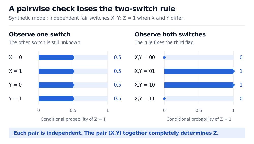
Conditional probabilities in a synthetic two-switch model. The probability that Z equals 1 is 0.5 given X alone or Y alone. Given both X and Y, it is 0, 1, 1, 0 for settings 00, 01, 10, 11. Each pair is independent even though both switches determine Z.
Original synthetic model, not market data. One observed switch leaves Z fair; observing both reveals its deterministic rule. All probabilities refer to the same scenario draw.
The three-way joint probability also fails the mutual-independence test:
P(X=1,Y=1,Z=1)=0=(21)3=81.
In this deliberately constructed generator, the third column is a label derived from the first two, not an additional random draw. Treating all three as independent fair inputs would generate impossible combinations such as 111. The pairwise tables cannot reveal this restriction on the full joint distribution.
A clean correlation matrix checks even less
Pairwise independent variables with finite second moments have zero pairwise covariance. That is enough for their variances to add in a sum. It is not enough to determine joint-event probabilities or the sum's full distribution.
There is a useful binary exception to the usual warning about covariance. For two 0–1 indicatorsI,J,
Cov(I,J)=P(I=1,J=1)−P(I=1)P(J=1).
If this is zero, the 11 cell factorises; subtracting it from the marginal probabilities forces the other three cells to factorise too. Thus zero population covariance is equivalent to independence for a pair of Bernoulli indicators, including deterministic boundary cases. If an indicator is constant, its Pearson correlation is undefined, despite its covariance being zero.
Outside this binary setting, zero covariance can miss dependence even between two variables. For example, let U take −1,0,1 with equal probabilities and set V=U2. Their covariance is zero by symmetry, although knowing U fixes V. Nor does a near-zero sample correlation establish a population property.
When validating a financial scenario generator, distinguish three claims: the marginal laws are appropriate; each pair has the intended relationship; and the whole collection has the intended joint law. Passing the second check does not establish the third. If a payoff depends on a combination of several flags, evaluate that combination under the joint model rather than multiplying marginal probabilities on the strength of pairwise checks.
For more worked detail, Independence — Example 6 treats the event version, while Covariance and Correlation develops the variance accounting. Both offer public previews; their full lessons require membership.
Sources
Dimitri P. Bertsekas and John N. Tsitsiklis, Introduction to Probability, 2nd edition (2008), §1.5, “Independence of a Collection of Events,” pp. 38–39, including Example 1.22; §2.7, “Independence of Several Random Variables,” p. 113. The stress-generator interpretation and conditional-probability figure are original.