Negative binomial distribution: Definition & Examples

The negative binomial distribution describes the number of failures before a fixed number of successes in independent Bernoulli trials, each with the same success probability. It also appears in a different role: modelling event counts whose variance exceeds their mean through a gamma–Poisson mixture. The distribution is the same; the economic assumptions behind these two constructions are different.

Fix the success target, let the attempts vary

Imagine a synthetic execution exercise in which each order attempt either fills one unit or fails. Attempts are independent, each fills with probability $p=0.25$ , and the exercise stops on the third fill. No partial fills, cancellations or changing market conditions enter this toy model.

Let

K

count failed attempts before the third fill. Its possible values are

0,1,2,\ldots

. Let

N

count all attempts up to and including that fill. Then

N=K+3

, so its possible values are

3,4,5,\ldots

More generally, for an integer target

r\ge 1

and

0<p<1

, the failures-count probability mass function is

\mathbb{P}(K=k)=\binom{k+r-1}{k}p^r(1-p)^k, \qquad k=0,1,2,\ldots.

Why that coefficient? The final attempt must succeed. Among the preceding

k+r-1

attempts, exactly

r-1

succeed and

k

fail. There are

\binom{k+r-1}{k}

ways to arrange those earlier outcomes. Independence supplies the product of their probabilities.

For two failures before the third fill, the stopping attempt is attempt five:

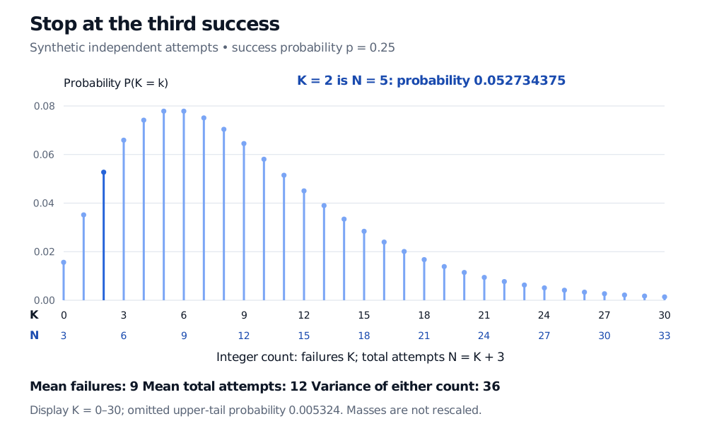
\mathbb{P}(K=2)=\mathbb{P}(N=5) =\binom{4}{2}(0.25)^3(0.75)^2 =0.052734375.

The coefficient is six because the first four attempts can arrange two successes and two failures in six ways. Using $\binom{5}{3}$ would incorrectly include sequences whose third success occurred before the final attempt.

Failure counts K from 0 to 30 and total attempts N from 3 to 33 share the same negative-binomial masses. With r=3 and p=0.25, K=2 is N=5 and has probability 0.052734375. Mean failures is 9, mean total attempts is 12, and either variance is 36.

Original synthetic stopping-count model. Filled points are probabilities at integer counts. The display ends at 30 failures; the omitted upper-tail mass is approximately 0.005324 and is not redistributed.

A binomial distribution fixes the number of attempts and counts successes. Here the success target is fixed and the stopping count varies. For

r=1

, the failures count reduces to the zero-based version of the geometric distribution; a geometric count starting at one instead counts the successful attempt as well.

Nine failures, twelve attempts

The attempts between successive successes are independent geometric waiting counts under the stated trial model. Their sum gives $N$ ; subtracting the $r$ successful attempts gives $K$ . Thus

\begin{aligned} \mathbb{E}[K]&=\frac{r(1-p)}{p}, &\mathbb{E}[N]&=\frac{r}{p},\\ \text{Var}(K)&=\frac{r(1-p)}{p^2}, &\text{Var}(N)&=\frac{r(1-p)}{p^2}. \end{aligned}

For the exercise, mean failures are 9, mean total attempts are 12, and either variance is 36 squared counts. Either standard deviation is 6 counts. Adding three changes the mean but leaves deviations around the mean unchanged.

These are model averages, not promised completion points. In particular, the probability of exceeding nine failures is approximately 0.390675. For a completion budget, a tail probability or quantile is more informative than the mean alone.

There is a useful bridge back to a fixed-trial binomial calculation. By attempt $k+r$ , the target has been reached exactly when at least $r$ successes have occurred:

F_K(k)=\mathbb{P}(K\le k) =\mathbb{P}\big(\operatorname{Binomial}(k+r,p)\ge r\big), \qquad k\ge0.

The 95% quantile is the smallest integer with cumulative probability at least 0.95. Here it is 20 failures:

F_K(19)\approx0.939351

while

F_K(20)\approx0.950797

. The corresponding total-attempt quantile is 23. This discrete threshold is not a fractional attempt obtained by interpolating the plot.

With $p=1$ , every attempt succeeds: $K=0$ and $N=r$ with certainty. With $p=0$ , the positive success target is never reached, so there is no proper finite stopping-count distribution. Real execution retries often have changing fill probabilities and dependence; the toy negative-binomial formula does not by itself establish a fill forecast.

A separate route: variable incident rates

Now change the question. Count operational incidents in a fixed period, rather than attempts until a fill target. A Poisson distribution with a fixed mean forces variance to equal that mean. A gamma-mixed Poisson model allows the latent period mean to vary:

C\mid\Lambda=\lambda\sim\operatorname{Poisson}(\lambda), \qquad \Lambda\sim\operatorname{Gamma}(r,\beta),

where

\beta>0

is a rate parameter, not a scale. Integrating over

\Lambda

gives the negative-binomial failures-form PMF with

p=\beta/(\beta+1)

. Here

r

is a gamma shape parameter and may be any positive real number; a noninteger shape has no literal interpretation as a target number of successes.

Writing the unconditional mean as $\mu=r/\beta=r(1-p)/p$ , the laws of total expectation and total variance give

\mathbb{E}[C]=\mu, \qquad \text{Var}(C)=\mu+\frac{\mu^2}{r}.

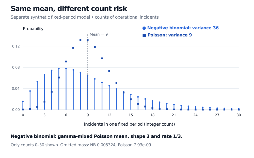
For a separate synthetic model with $r=3$ and $\beta=1/3$ , the gamma-distributed period mean has mean 9 and variance 27. The resulting incident count has mean 9 and variance $9+27=36$ , whereas a fixed-mean Poisson count with mean 9 has variance 9.

Synthetic fixed-period incident counts compare a negative binomial with mean 9 and variance 36 against a Poisson with mean 9 and variance 9. The negative binomial is broader, with more mass at very low counts and in the far right tail. The shared mean is marked at 9.

Original fixed-period illustration. The negative binomial arises from a gamma-mixed Poisson mean with shape 3 and rate 1/3. This is a different modelling story from stopping after three successful attempts.

This construction explains overdispersion, but observed variance above the mean does not identify a gamma mixture. Dependence, exposure differences or other heterogeneity can also create excess variation. A negative-binomial count model also says nothing about incident severity: monetary losses require an additional loss-size model. Under fixed

\mu

, increasing

r

reduces the extra variance and approaches a Poisson law.

For the geometric moment building blocks, see Means and Variances of the Named Distributions. For the separate risk application, The Loss Distribution Approach, §5, develops Poisson mixtures before combining frequency with severity. Both have public previews; full lessons require membership.

Sources

Dimitri P. Bertsekas and John N. Tsitsiklis, Introduction to Probability, 2nd edition (2008), §6.1, “The kth Arrival Time”: geometric-sum and Pascal waiting-count construction.
Alexander J. McNeil, Rüdiger Frey and Paul Embrechts, Quantitative Risk Management: Concepts, Techniques and Tools, revised edition (2015), §13.2.4, Proposition 13.21: negative binomial as a gamma–Poisson mixture.
R Core Team, stats: The Negative Binomial Distribution: failures convention, mean–dispersion parameterisation and smallest-integer quantiles.

Fix the success target, let the attempts vary

Nine failures, twelve attempts

A separate route: variable incident rates

Sources

Related terms

Bernoulli distribution

Binomial distribution

Geometric distribution

Mutual independence

Poisson distribution

Probability mass function

Quantile