Hypergeometric distribution: Definition & Examples

The hypergeometric distribution gives the number of items with a specified label in a uniform random sample drawn without replacement from a finite population whose label counts are fixed. It answers questions such as: if an order-audit pool contains a known number of flagged records, how likely is a random inspection to include at least one?

The randomness is in which records are sampled. The labels in the pool are already fixed. This is a different experiment from generating new, independent flags with a constant probability on each trial.

Count the samples, not independent successes

Let $N$ be the population size, $K$ the number of labelled items and $n$ the sample size. Assume integers $N\ge1$ , $0\le K\le N$ and $0\le n\le N$ . If every $n$ -item subset is equally likely and $X$ counts labelled items in the sample, write

X\sim\operatorname{Hypergeometric}(N,K,n).

Its probability mass function is

\mathbb{P}(X=x)=\frac{\binom{K}{x}\binom{N-K}{n-x}}{\binom{N}{n}}, \qquad \max(0,n-(N-K))\le x\le\min(n,K),

for integer

x

, and zero elsewhere. The denominator counts all samples; the numerator chooses

x

labelled items and

n-x

unlabelled items. No ordering factor is needed: both counts concern unordered subsets. The Counting and Combinatorics lesson develops this subset interpretation of the binomial coefficient; the public page is a preview and the full lesson requires membership.

The support has two constraints that are easy to miss. You cannot draw more than

K

labelled items, and you cannot draw more than

N-K

unlabelled items. For example, with 20 records and 5 flags, a sample of 17 must contain at least 2 flags: only 15 unflagged records exist. The support is then

2,3,4,5

, rather than every count from zero to 17. Penn State's STAT 414 notes introduce the law through the same two-category sampling structure.

A four-order inspection

Consider a synthetic audit-design scenario: a frozen pool has 20 order records, exactly 5 of which carry a particular surveillance flag. Select 4 distinct records uniformly at random. A flag is a label for inspection, not proof of a trading violation. We condition on the stipulated pool composition; we are not estimating how many flags exist.

There are $\binom{20}{4}=4{,}845$ possible samples. A clean sweep of four unflagged records occurs in $\binom{15}{4}=1{,}365$ of them, so

\mathbb{P}(X=0)=\frac{\binom{15}{4}}{\binom{20}{4}} =\frac{91}{323}\approx0.281734.

Using the complement rule, the probability of finding at least one flag is

\mathbb{P}(X\ge1)=1-\frac{91}{323} =\frac{232}{323}\approx71.8266\%.

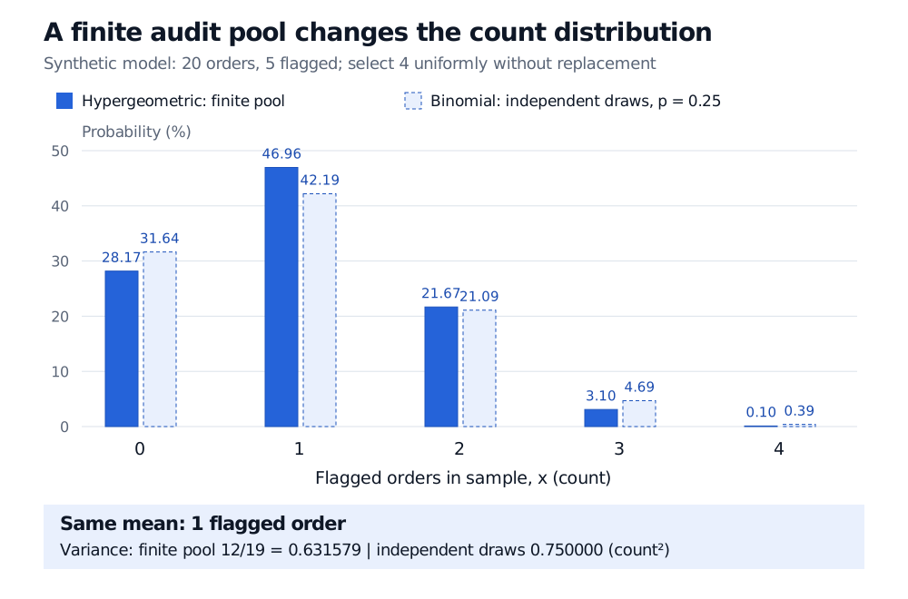
The whole distribution shows what that detection probability contains:

Flags in sample, $x$	Samples with this count	Probability
0	1,365	28.1734%
1	2,275	46.9556%
2	1,050	21.6718%
3	150	3.0960%
4	5	0.1032%

Percentages are rounded individually. A mean count of one does not mean every inspection finds one: both zero and multiple flags have positive probability.

Paired probability bars compare a synthetic hypergeometric sample of 4 orders from 20 with 5 flags against four independent draws with flag probability 0.25. Both means are 1. Finite-pool variance is 0.631579 count squared versus 0.75 for independent draws; zero-flag probabilities are 28.17% and 31.64%.

Original synthetic sampling model. Solid bars use a fixed pool without replacement; outlined bars use independent binomial trials with the same marginal flag probability. The plotted distribution is a count of labels, not a distribution of financial losses.

Equal marginal probabilities, dependent draws

Before looking at any results, each draw position has flag probability $5/20=1/4$ . Yet observing the first draw changes the composition left for the second:

\begin{aligned} \mathbb{P}(\text{second flagged}\mid\text{first flagged})&=\frac4{19},\\ \mathbb{P}(\text{second flagged}\mid\text{first unflagged})&=\frac5{19}. \end{aligned}

Neither conditional probability equals

1/4

. Thus the flag indicators are identically distributed across draw positions but lack independence. The Conditional Probability lesson, available as a public preview with full text for members, builds the multiplication rule used here. For example, the zero-flag probability can also be calculated sequentially as

\frac{15}{20}\frac{14}{19}\frac{13}{18}\frac{12}{17}=\frac{91}{323}.

Let

p=K/N

. The expected value is

\mathbb{E}[X]=np

, because expectation adds the

n

indicator means even when the indicators are dependent. For

N>1

, the variance is

\text{Var}(X)=np(1-p)\frac{N-n}{N-1}.

The factor

(N-n)/(N-1)

is the finite population correction to the binomial variance. For standard deviation, take its square root. In our example,

\mathbb{E}[X]=4\left(\frac14\right)=1, \qquad \text{Var}(X)=4\left(\frac14\right)\left(\frac34\right)\frac{16}{19} =\frac{12}{19}\approx0.631579.

The units are flagged-order counts for the mean and squared counts for variance. To see why dispersion falls, let $I_i$ indicate a labelled item at draw position $i$ . For distinct positions in a sample of at least two items,

\text{Cov}(I_i,I_j)=-\frac{p(1-p)}{N-1}.

Drawing one labelled item depletes the supply available for the others. Summing $n$ individual variances and $n(n-1)$ ordered covariance terms gives the correction. When the entire population is sampled, $n=N$ and $X=K$ with certainty. For $N=1$ , handle the single-item population directly: every allowed sample count is deterministic, so variance is zero rather than an undefined $0/0$ calculation.

When a binomial approximation changes the answer

A binomial distribution with parameters

n

and

p=K/N

has the same mean but assumes independent trials. In this example it gives variance

4(1/4)(3/4)=0.75

and

\mathbb{P}_{\text{binomial}}(X\ge1)=1-\left(\frac34\right)^4 =\frac{175}{256}\approx68.3594\%.

That is below the exact finite-pool detection probability of 71.8266%. Lower variance does not mean every tail probability falls; here zero flags becomes less likely, raising the probability of at least one.

For fixed $n$ , as $N$ grows and $K/N$ approaches a fixed proportion, the hypergeometric law approaches the corresponding binomial law. In practical approximation work, inspect the sample fraction and the event being calculated. A small variance correction alone does not certify accurate relative probabilities for a rare event or for counts near a finite-support boundary.

Uniform selection is essential. A risk-weighted audit that deliberately oversamples suspicious orders does not generally follow this law. Nor does a portfolio's future default count become hypergeometric merely because there are finitely many names: future labels may be random, heterogeneous and dependent through economic conditions. If $K$ is unknown, the formula is conditional on each proposed $K$ ; inference about $K$ requires an additional statistical argument.

For software calculations, verify the parameter convention. In R's official hypergeometric documentation, m and n are the labelled and unlabelled population counts, while k is the sample size. Its upper-tail option returns a strict exceedance probability, so the threshold must reflect whether the question says “more than” or “at least.”

Sources

Sheldon M. Ross, A First Course in Probability, 10th edition, §4.8.3, “The Hypergeometric Random Variable,” especially equation (8.4) and Example 8j; sampling-without-replacement law, binomial approximation and moments.
Penn State, STAT 414, §7.4: Hypergeometric Distribution — two-category sample counting and support constraints.
R Core Team, stats: The Hypergeometric Distribution — parameter conventions, support, moments, cumulative probabilities and quantiles.

Count the samples, not independent successes

A four-order inspection

Equal marginal probabilities, dependent draws

When a binomial approximation changes the answer

Sources

Related terms

Binomial distribution

Complementary event

Expected value

Independence

Indicator function

Probability mass function

Variance