A random vector describes uncertain quantities together. Follow a three-state asset-return model from its joint law to its mean, covariance matrix and portfolio risk.
Random vector
A random vector is an ordered collection of random variables defined on the same probability space. One outcome determines all its components together. A portfolio's uncertain asset returns form a random vector; the portfolio weights chosen before the period can be an ordinary fixed vector.
A random vector need not describe a time series: its coordinates might be different assets at one future date. A finite selection of observations from a stochastic process can also form a random vector, but the process itself is a time-indexed collection.
A scenario selects a pair, not two separate draws
Suppose a synthetic model specifies the simple total returns of assets A and B over the same one-month period, on a common currency basis. The three states are exhaustive within this model; their probabilities are stipulated, not estimated market frequencies. Coordinate order is always (A,B).
State
Model probability
A return
B return
50/50 portfolio return
S1
0.50
2%
1%
1.5%
S2
0.30
−1%
3%
1.0%
S3
0.20
4%
−2%
1.0%
Thus R=(RA,RB)T takes the decimal-return values (0.02,0.01)T, (−0.01,0.03)T and (0.04,−0.02)T. If S2 occurs, the realised vector is (−0.01,0.03)T: A's loss and B's gain belong to the same scenario.
For example, pR(0.02,0.01)=0.50. The marginal distributions separately give P(RA=0.02)=0.50 and P(RB=0.01)=0.50. Their product is 0.25, so these components are not independent. Drawing the two marginals independently would replace this joint model with a different one and introduce return pairs absent from the table.
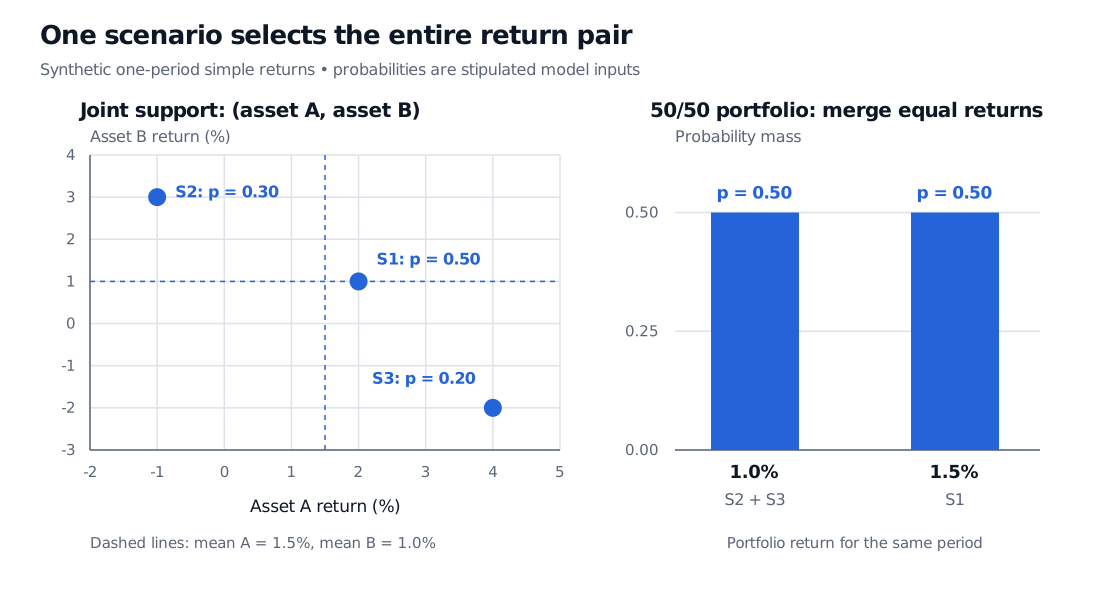
Three filled points show one-month return pairs in percent: S1 is (2,1) with probability 0.50, S2 is (−1,3) with probability 0.30, and S3 is (4,−2) with probability 0.20. Dashed lines mark means (1.5,1.0) percent. The 50/50 portfolio has return 1.0% with combined probability 0.50 and 1.5% with probability 0.50.
Original synthetic one-month simple-return model. Left: one filled point per joint state. Right: S2 and S3 give the same portfolio return, so their probabilities add.
Mean vector and covariance matrix
When each component has a finite absolute first moment, take expectations component by component:
μ=E[R]=(E[RA]mathbbE[RB])=(0.0150.010).
For example, E[RA]=0.50(0.02)+0.30(−0.01)+0.20(0.04)=0.015. The mean vector is not itself a possible return pair in this model. It summarises the law rather than predicting which scenario will occur.
With finite second moments, the covariance matrix is
These are squared decimal-return units. If both returns are instead entered numerically in percentage points, every matrix entry is multiplied by 1002=10,000: the covariance becomes −3 percentage-points squared. Changing units does not change the economic exposure.
A covariance matrix is symmetric and positive semidefinite: for every fixed vector a, aTΣa=Var(aTR)≥0. It may be singular. A random vector can exist even when these moments are infinite or undefined, in which case this finite-matrix summary is unavailable. Even when they exist, mean and covariance generally do not specify the full joint law, particularly its tail behaviour.
Turn the vector into a portfolio return
Allocate half the initial capital to each asset, hold the positions through the month, and ignore trading costs and external cash flows. With fixed period-start weights w=(0.5,0.5)T, the portfolio's simple return is
Rp=wTR=0.5RA+0.5RB.
This gives the three portfolio returns in the table. Their probability-weighted mean is 0.50(0.015)+0.30(0.010)+0.20(0.010)=0.0125, or 1.25% over the month. Matrix notation gives the same answer: E[Rp]=wTμ.
Its standard deviation is 0.00000625=0.0025, or 0.25 percentage points for this month. Directly from the two distinct portfolio returns, the variance is also 0.50(0.015−0.0125)2+0.50(0.010−0.0125)2. The negative covariance offsets much of the standalone variance contribution; setting it to zero would change the calculation. MIT's finance mathematics lecture derives these linear-combination formulas.
These are population moments of the stated finite model, not sample estimates from three historical months. There is no sample-size divisor or automatic annualisation. The positive portfolio return in every listed state is a feature of this synthetic scenario set; it does not establish a guaranteed investment opportunity in actual markets.
Before using vector arithmetic in a risk system, keep coordinate labels and units attached to the data. Reordering returns requires reordering weights and covariance rows and columns consistently. Combining a daily A return with a monthly B return, or treating one component as a percentage while the other is a decimal, changes what the calculation means. The weighted-simple-return identity also needs its stated exposure convention; a weighted sum of asset log returns is generally not the portfolio's log return.
For a slower introduction to the scalar moments used here, read Expectation, Variance and Covariance, available in full with a free signed-in account.
Sources
Dimitri P. Bertsekas and John N. Tsitsiklis, Introduction to Probability, 2nd edition, Athena Scientific, 2008, §2.5 (joint PMFs of multiple random variables) and §4.2 (covariance, correlation and variance of sums).