Understand conditional expectation as an information-based mean, distinguish a random forecast from its observed value, and split forecast error into within-regime and between-regime variation.
Conditional expectation
Conditional expectation is the mean of a random variable using specified information. For a future trading profit or loss X, it answers: what is the probability-weighted average P&L among the possibilities consistent with what I know?
The answer depends on both the information and the probability model. A forecast given tomorrow's market regime differs from one made before the regime is known. Neither forecast is a promised cash flow, and neither needs to be an outcome the trade can actually produce.
A forecast that changes when the regime is revealed
Consider a synthetic one-period trading P&L, measured in USD. Let Y identify a calm or stress regime. The regime is observed before the final P&L, with these stipulated probabilities:
Regime
Regime probability
Possible P&L, conditional on regime
Conditional mean
Conditional variance
Calm
0.75
0 or 4, each with probability 0.5
USD 2
4 USD²
Stress
0.25
−10 or 2, each with probability 0.5
USD −4
36 USD²
Before observing the regime, the forecast is
E[X]=0.75(2)+0.25(−4)=0.50 USD.
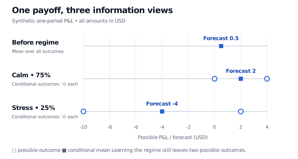
After observing calm, use the calm distribution: (0+4)/2=2. After observing stress, use the stress distribution: (−10+2)/2=−4. The stress forecast is negative even though a positive P&L remains possible.
Here is the distinction hidden in the notation:
E[X∣Y]=g(Y),g(y)={2,−4,y=calm,y=stress.
E[X∣Y] is a random variable before Y is observed. It will take the value 2 or −4. In contrast, E[X∣Y=calm]=2 is a number evaluated at a specified regime. A forecast can be random because its eventual information is random.
Synthetic one-period P&L in USD. Before the regime is known the mean is 0.50. Calm has probability 0.75, outcomes 0 and 4, and mean 2. Stress has probability 0.25, outcomes −10 and 2, and mean −4. Each conditional outcome has probability one half.
Original synthetic regime model. Circles show possible final P&Ls; squares show mean forecasts. Observing the regime selects a row, but leaves two possible outcomes.
The forecast 2 happens to equal one possible outcome in the overall model, but the calm trade itself pays only 0 or 4. An expectation averages outcomes; it does not choose the most likely one.
What goes to the right of the bar?
For discrete X and Y, at a value y with positive probability,
E[X∣Y=y]=x∑xP(X=x∣Y=y).
The probabilities in this sum must add to one within the specified condition. In the example, the joint probability of calm and P&L 4 is 0.75×0.5=0.375. Its conditional probability given calm is 0.375/0.75=0.5. Using 0.375 inside the conditional average would fail to renormalise the remaining possibilities.
When a joint density exists, the analogous calculation is
E[X∣Y=y]=∫−∞∞xfX∣Y(x∣y)dx.
For a continuously distributed Y, an exact event Y=y has probability zero. The density formula defines a conditional mean without dividing event probabilities by zero; its values are determined only up to sets of Y-probability zero. A conditional density is a computational representation when available, not a requirement for the general concept.
More generally, write E[X∣G], where G is a collection of observable events, formally a sigma-algebra. If X is integrable, meaning E[∣X∣]<∞, the conditional expectation is the integrable random variable Z satisfying
Z is G-measurable,E[Z1A]=E[X1A]for every A∈G.
Measurability means the available information determines the forecast. The second condition means it preserves the original probability-weighted total inside every observable event. These conditions determine Z up to events of probability zero. Gravner's university notes give this definition and the associated information rules.
Average the revised forecasts to recover the original
The tower property, also called the law of iterated expectations, says
E[E[X∣Y]]=E[X].
The calm and stress forecasts average to USD 0.50 using probabilities 0.75 and 0.25. An unweighted average of 2 and −4 would give −1 and answer a different question: it would implicitly treat the regimes as equally likely. Gravner's introductory probability notes, Theorem 8.3 derive the weighted identity.
For nested information sets H⊆G,
E[E[X∣G]∣H]=E[X∣H].
Forecast with richer information, then average back using less information, and you recover the less-informed forecast. A filtration organises such information through time. Consequently, conditional forecasts of a fixed integrable payoff form a martingale under that information and probability measure. This is a consistency property of the model; an estimated forecasting rule can still be wrong.
Learning the regime leaves risk inside each regime
The conditional mean says little about the spread of outcomes by itself. Here calm outcomes lie 2 dollars either side of their mean, giving variance 4 USD². Stress outcomes lie 6 dollars either side of −4, giving variance 36 USD². Observing stress actually reveals a more dispersed conditional distribution than the original mixture.
For finite second moments, the law of total variance separates two contributions:
Var(X)=E[Var(X∣Y)]+Var(E[X∣Y]).
In this example, the average variance remaining within regimes is
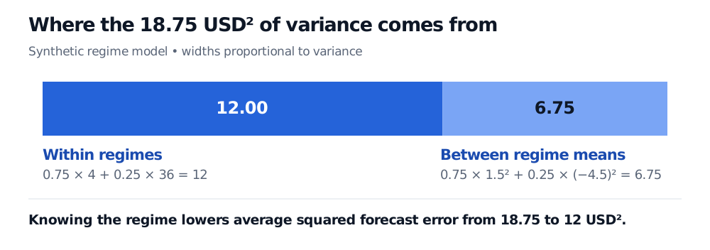
0.75(4)+0.25(36)=12 USD2.
The variance of the regime means around the overall mean is
A proportional variance bar shows total P&L variance 18.75 USD squared split into 12 of within-regime variance and 6.75 of variance between regime means. Regime-aware mean-squared forecast error is 12.
Original synthetic variance decomposition. Knowing the regime removes uncertainty about which conditional mean applies; uncertainty within the chosen regime remains.
This does not say that every realised information update lowers conditional variance. Stress variance is 36, exceeding 18.75. The reduction is in average squared forecasting error across the model's possible information outcomes.
Why the mean is a useful forecast—and where it stops
With finite second moments, m(Y)=E[X∣Y] minimises expected squared error among square-integrable forecasts using only Y. For any such competing forecast h(Y),
E[(X−h(Y))2]=E[(X−m(Y))2]+E[(m(Y)−h(Y))2].
The last term cannot be negative. In the regime model, always forecasting USD 0.50 gives mean-squared error 18.75 USD². Using 2 in calm and −4 in stress reduces it to 12 USD². The remaining error has conditional mean zero, but it need not be independent of the regime: its spread here plainly depends on the regime.
This optimality concerns squared-error loss under the specified model. It does not guarantee profitable trades, identify the best action under asymmetric losses, or make an arbitrary linear regression equal the true conditional mean. A fitted model estimates the target and can omit relevant information or use unstable relationships.
The probability measure also matters. A physical conditional mean is a model of average outcomes under physical probabilities. In risk-neutral pricing, the discounted payoff is averaged under a pricing measure justified by market assumptions. Conditioning on information does not itself convert a statistical forecast into a fair derivative price.
For a fuller treatment, the SelfMadeQuant Conditional Expectation lesson develops the tower property, factor forecasts, variance decomposition and squared-error argument. Its public page is a preview; the full lesson requires membership.
Sources
Joseph K. Blitzstein and Jessica Hwang, Introduction to Probability, 2nd edition, §§9.1–9.3 (conditioning, tower and projection interpretation), §9.4 (squared-error geometry), and §9.5, Theorem 9.5.5 (total variance). Regime scenarios and figures are original.
Steven E. Shreve, Stochastic Calculus and Finance, Carnegie Mellon lecture notes, Prasad Chalasani and Somesh Jha, 25 July 1997, §§2.3.2–2.3.4 (information-based definition, uniqueness and tower property). This is the lecture-note text, not the later Volume I textbook.