Measure observed return variation, calculate annualised historical volatility, and distinguish centred sample estimates from uncentred realised variance.
Realised volatility
Realised volatility measures how much an asset's returns varied over an observed period. It is calculated from prices or returns that have already occurred. Traders use it to describe recent market movement, evaluate volatility forecasts and compare historical movement with the volatility embedded in option prices.
The label alone does not identify a unique calculation. A historical standard deviation usually subtracts the sample mean; a common realised-variance measure sums squared returns without subtracting it. Frequency, window, return definition and annualisation also matter. CME's introduction describes the familiar historical standard-deviation approach and the choice of observation window.
A stock can finish higher and still have a rough week
A risk analyst receives six consecutive daily closing observations for a fictional stock. Construct them from an initial price of 100 and these five daily log returns:
r=(−0.02,0.01,0.03,−0.01,0.02).
The corresponding prices, rounded only for display, are:
Observation
0
1
2
3
4
5
Synthetic price
100.0000
98.0199
99.0050
102.0201
101.0050
103.0455
These are constructed data, with no dividends or corporate actions. A log return is
ri=ln(Pi−1Pi).
Thus six prices give five returns, not six. A return of 0.02 means a log return of 2%; the corresponding simple return is e0.02−1, which is slightly larger than 2%. Keep decimal inputs throughout the variance calculation.
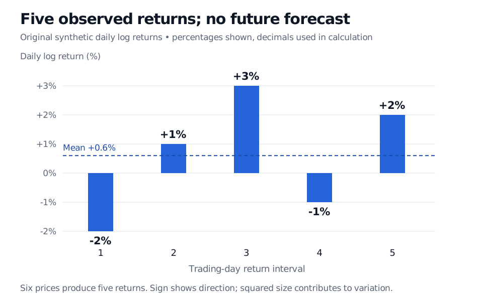
Five synthetic daily log returns: minus 2%, plus 1%, plus 3%, minus 1%, plus 2%, around a mean of plus 0.6%. Six prices give five returns.
Original synthetic observations. The vertical axis shows daily log returns in percent; calculations use decimals.
The stock's cumulative log return is 0.03, so its cumulative simple return is e0.03−1≈3.05%. That says where it finished. Volatility describes the variation along the way. Squaring makes a large negative move contribute just as much as a positive move of the same size to an uncentred measure. Volatility is not a directional forecast.
The centred historical estimate, step by step
For n equally spaced daily log returns, define the mean and sample daily variance as
rˉ=n1i=1∑nri,sd2=n−11i=1∑n(ri−rˉ)2.
This is the standard historical calculation in Hull's §15.4. The divisor n−1 accounts for estimating the mean from the same observations. Under independent, identically distributed returns with finite variance, it makes sample variance unbiased for the common daily variance. Taking the square root does not make the resulting standard deviation exactly unbiased.
For our five returns,
rˉ=0.006,∑ri2=0.0019,∑(ri−rˉ)2=0.00172.
The last number can also be checked as 0.0019−5(0.006)2. Therefore
sd2=40.00172=0.00043,sd=0.00043≈0.0207364.
The daily sample standard deviation is 2.0736%. Stipulating 252 trading days per year, its conventional annualised quotation is
σ^hist=252sd=252×0.00043≈0.3291808=32.92%.
Variance scales by 252; standard deviation scales by 252. The annualised variance here is 0.10836 in squared decimal-return units per year. Its square root is 0.3291808 in decimal-return units per square-root year, conventionally quoted as 32.92% annual volatility. Neither number is the five-day cumulative return.
For help with the statistical foundation, Basic Statistics and Regression, available in full with a free signed-in account, explains sample variance and why standard deviation differs from the standard error of an estimated mean.
Why another screen might show 30.95%
Another analyst uses an uncentred realised-variance convention. Over this five-trading-day window, first add the squared daily log returns:
RVwindow=i=1∑nri2=0.0019.
To quote an annualised rate of variation, divide by the window's stipulated length n/252 trading years:
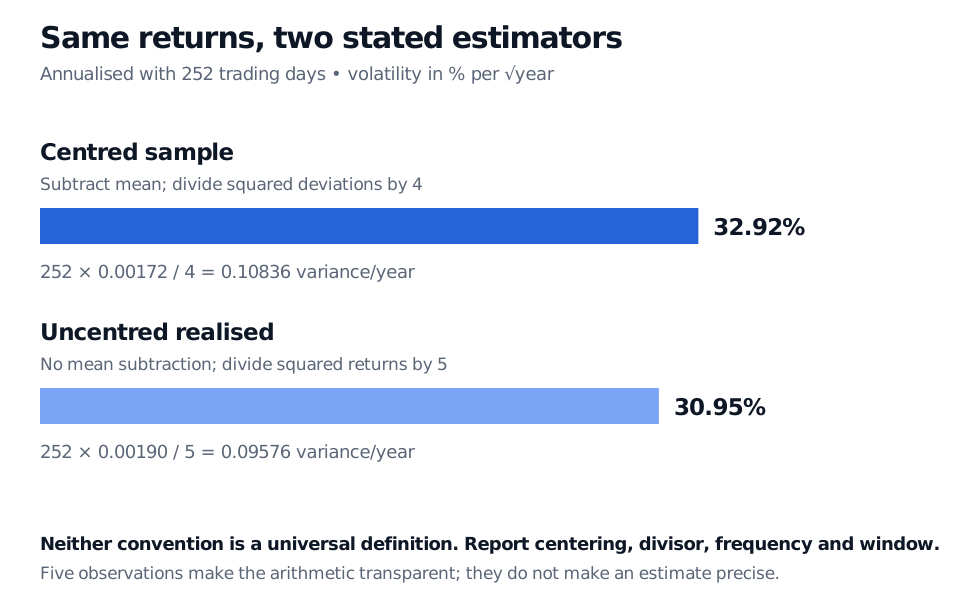
The same five returns give centred sample annualised variance 0.10836 and volatility 32.92%, versus uncentred annualised realised variance 0.09576 and volatility 30.95%. Mean subtraction and divisors differ.
Same synthetic returns; 252 trading days per year. Variance uses squared decimal returns per year, while volatility is displayed in percent per square-root year.
Both the centering and divisor changed. Removing the mean reduces the numerator, but dividing by four rather than five raises the sample estimate enough to reverse their order here. Neither number is the universal correct definition of “realised volatility.” If a variance swap settles against realised variance, the contract's observation and annualisation rules control its settlement measure.
The uncentred construction also has a distinct theoretical role. With increasingly fine observations of an ideal frictionless log-price process, sums of squared returns approach its quadratic variation. A continuous diffusion contributes integrated instantaneous variance; jumps add squared log-price jumps. At very high frequency, bid–ask bounce and other microstructure noise can contaminate the estimate. Andersen and Bollerslev explain these connections and limitations in equations 25 and 28. Five daily observations do not deliver that limiting object exactly.
What must accompany a reported number
A useful report identifies the underlying series, return basis, sampling times, window, estimator and annualisation. These choices resolve many apparent disagreements:
Price or total return? A raw close-to-close price series includes the price drop at an ex-dividend date. A properly constructed total-return series includes the distribution; split adjustments prevent artificial price jumps. Use the series appropriate to the question and verify the vendor's adjustment definition. An “adjusted close” label alone is insufficient; do not mix raw prices with an adjusted series midway through a window.
Which intervals? Daily closes include overnight movement. Intraday open-to-close sampling omits it unless it is added explicitly. Different closing times, missing observations and irregular intervals alter the measurement; a missing close is not a zero return.
Which window? A short rolling window responds quickly but is noisy. A long one pools more data but can mix different volatility regimes. A rolling spike can also disappear when one large return leaves the window. Five observations here teach arithmetic, not reliable precision.
Which clock? We stipulated 252 trading days. A market trading every calendar day may use a different convention. The multiplier must match the data frequency. Square-root-time scaling as a statement about future cumulative-return uncertainty requires assumptions such as stable daily variance and zero serial covariance; annualising an observed statistic does not establish them.
Realised volatility is an observation-based input to risk work. Implied volatility is inferred from an option price using a pricing model. Comparing today's option-implied number with a trailing historical window mixes a future option horizon with a past sample. A forecast of the future matched period is needed for that comparison; volatility risk premia, model assumptions and costs also matter. A historical estimate alone does not establish that an option is cheap or expensive.
Check your convention
1. Three daily log returns are (−0.01,0,0.01). Using 252 trading days, calculate annualised volatility both as a centred sample standard deviation and as the square root of annualised uncentred realised variance. Why do the answers differ even though the mean is zero?
Answer. The mean is zero and the squared-return sum is 0.0002. The centred sample daily variance is 0.0002/2=0.0001, so annualised volatility is 252(0.0001)≈15.87%. The uncentred annualised variance is (252/3)(0.0002)=0.0168, giving volatility 0.0168≈12.96%. Centering makes no difference here; the divisors two and three do.
2. A stock has the same positive daily log return, 0.01, on each of three days. Must both estimators be zero because the path is smooth?
Answer. No. The centred sample variance is zero because every return equals its mean. The uncentred squared-return sum is 3(0.01)2=0.0003, which is positive. A constant positive return has direction without sample dispersion. At a finite sampling frequency, the two estimators need not assign the same value to it.
Sources
John C. Hull, Options, Futures, and Other Derivatives, 9th Global Edition, §15.4, “Estimating Volatility from Historical Data,” pp. 348–350 — log returns, sample standard deviation, annualisation and dividend treatment. All prices, return sequences, calculations and figures here are original synthetic examples.