Quadratic variation is the limit of squared-increment sums. Derive Brownian moments, separate path roughness from endpoint variance, and see why drift vanishes but Itô corrections survive.
Quadratic variation
Quadratic variation is the limit of sums of squared changes in a process as the observation intervals shrink. For a continuous diffusion, it records the accumulated contribution of the random shocks. A smooth trend contributes zero, even when that trend produces a large change from start to finish.
This is why an option's curvature matters in stochastic calculus: squared price changes can survive the continuous-time limit. They generate the extra term in Itô's lemma, rather than disappearing as they do along a smooth path.
The notation [X]T, also written [X,X]T, means quadratic variation accumulated from time zero to T.
First specify the grid and the limit
Choose a deterministic partition π={0=t0<t1<⋯<tn=T} and calculate
The mesh∣π∣ is the longest observation interval. Refinement must make this longest interval tend to zero; adding observations near the beginning while leaving a large gap at the end is insufficient.
For a continuous semimartingale, these sums converge in probability to [X]T as the deterministic mesh vanishes. Convergence in probability means that the probability of an error larger than any fixed positive tolerance tends to zero. It does not say that every finite-grid sum equals the limit. This probability-limit formulation is the general setting behind the quadratic variation of continuous local martingales. Dey's Lecture 12 gives the local-martingale construction.
Quadratic variation is not the supremum of these squared sums over every possible partition. The choice of partitions and the mode of convergence belong in the statement.
Brownian motion: the calculation that makes the limit work
For standard Brownian motion, an increment over an interval of length hi is hiZi, with independent standard normal variables Zi. Since E[Zi2]=1 and E[Zi4]=3,
E[Qπ(W)]=T,Var(Qπ(W))=2i∑hi2≤2T∣π∣.
Therefore
E[(Qπ(W)−T)2]⟶0.
This is mean-square, or L2, convergence, which also implies convergence in probability. The resulting identity is [W]T=T. Lawler's §2.8 develops this moment calculation and the partition conditions.
On a uniform grid with n intervals,
E[Qn(W)]=T,Var(Qn(W))=n2T2.
For T=1 in the chosen Brownian time unit:
Number of intervals n
Mean of Qn
Standard deviation of Qn
4
1
0.707107
16
1
0.353553
256
1
0.088388
The mean is exactly one at every resolution. An individual path's sum is random, and only becomes concentrated around one as resolution increases.
For fixed dyadic grids—successively halving each interval—the convergence also holds almost surely. That is a statement about a specified grid sequence on an event of probability one, rather than a guarantee covering every partition sequence someone might select after seeing the whole path. See Lalley's §5. Appropriately controlled stopping-time sampling also has a place in the broader theory; a random partition is not automatically invalid.
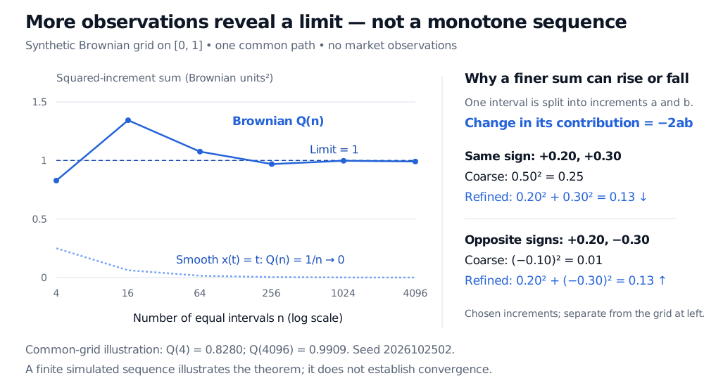
Nested squared-increment sums from one synthetic Brownian grid fluctuate around the limit 1: 0.8280 at 4 intervals and 0.9909 at 4096. The smooth path x(t)=t has sums 1/n tending to zero. Splitting same-sign increments lowers their squared contribution from 0.25 to 0.13; splitting opposite-sign increments raises it from 0.01 to 0.13.
Original synthetic illustration, seed 2026102502, with all coarser Brownian grids aggregated from the same 4096 increments on [0,1]. The separate split examples show why a finite sum can rise or fall. A finite simulation illustrates the limit theorem; it does not prove it.
Indeed, splitting a coarse increment a+b into a and b changes its contribution by
a2+b2−(a+b)2=−2ab.
Same-sign subincrements reduce the sum; opposite signs increase it. More observations need not produce a monotone approach to the limit.
A trend can move far and contribute nothing
Take the smooth path xt=t. On a uniform grid over [0,T],
Qn(x)=n(nT)2=nT2⟶0.
At T=1, the path has moved by one unit, yet its quadratic variation is zero. Quadratic variation measures accumulated squared fluctuation at fine scales, rather than net displacement.
More generally, a continuous finite-variation path has zero quadratic variation. The continuity qualification matters: a jump of size J contributes J2. For example, a Poisson process has unit jumps and [N]T=NT, despite having finite total variation on each finite horizon. Brownian paths have infinite total variation and finite quadratic variation; these are different notions of variation. Baudoin's Lecture 15 proves the Brownian contrast.
Nor is quadratic variation the variance of the level at a date. Suppose Xt=Zt, where a fair coin chooses Z=+1 or −1 once at the start. Every realised path is a straight line, so [X]T=0, but Var(XT)=T2. Endpoint variance compares possible outcomes across paths; quadratic variation accumulates squared changes along a path through time.
Reading the number in a financial model
Consider a synthetic log-price model, with time in years,
Lt=log(St/S0)=at+0.30Wt.
Here a is a constant log drift per year and 0.30 is the diffusion loading in log points per square-root year. Its quadratic variation is
[L]T=0.302T=0.09T.
Over one year the limit is 0.09 squared log points. Dividing by the one-year horizon gives an annual variance rate of 0.09; its square root is annual volatility 30%. Adding a larger constant drift changes the path's trend but leaves this quadratic variation unchanged.
At finite resolution, drift does contribute to the expected raw squared sum:
E[Qn(L)]=0.09T+na2T2.
With a=0.08, T=1 and n=256, this expectation is 0.090025, while the quadratic-variation limit remains 0.09. A finite sum is an estimator of the limiting quantity; its expectation need not equal that quantity. Taking a square root introduces a further nonlinear transformation, so unbiasedness of a variance estimator would not imply unbiasedness of its volatility estimate.
For a continuous Itô model dXt=atdt+btdWt, under the usual adaptedness and local integrability conditions,
[X]T=∫0Tbt2dt.
This can itself be random when the diffusion loading is random. For log prices it is integrated variance; for a price measured in dollars, quadratic variation has dollar-squared units instead. Always identify the process being sampled. Observed market quotes, jumps and observation error require a measurement model before interpreting a finer-grid sum as diffusion variance.
The correction ordinary calculus would miss
On every finite grid, the algebraic identity
WT2=2i∑Wti−1(Wti−Wti−1)+Qπ(W)
holds exactly when W0=0. Passing to the appropriate limits yields
∫0TWtdWt=21(WT2−T).
The last term is the accumulated quadratic variation. Omitting it would give the wrong Itô integral. In option pricing, the same surviving second-order contribution couples variance with gamma: curvature converts small random price movements into a term that ordinary smooth-path calculus discards.
Gregory F. Lawler, Stochastic Calculus: An Introduction with Applications, revision dated 15 February 2023, §2.8, Theorems 2.8.1–2.8.2; §3.2, Theorem 3.2.6 and equation (3.8). Grounding text for the partition moments, drift invariance and stochastic-integral identities.