Itô integral: Definition & Examples

The Itô integral accumulates a changing exposure to random shocks while requiring that each exposure be chosen using information available before the corresponding shock. With Brownian motion

W_t

as the noise source, it is written

I_t=\int_0^t H_s\,dW_s.

Here

H_s

is the exposure, or integrand. In finance, this is the mathematical building block for the random part of a trading gain. The integration rule matters: moving the exposure from the beginning to the end of each interval changes the result.

Hold first, observe second

Start with a strategy that changes only at fixed times $0=t_0<\cdots<t_n=T$ . On the interval from $t_j$ to $t_{j+1}$ , hold $H_j$ , chosen from the information $\mathcal F_{t_j}$ . Then the integral has an explicit definition:

\int_0^T H_s\,dW_s =\sum_{j=0}^{n-1}H_j\left(W_{t_{j+1}}-W_{t_j}\right).

The filtration

(\mathcal F_t)

describes available information, and

W

must be Brownian motion relative to it. In particular, its next increment is independent of the current information. You may change your position after observing a move; you cannot retroactively apply the new position to that move.

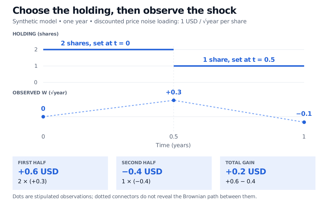
Consider a hypothetical asset whose discounted price is driven only by Brownian noise, with coefficient one USD per square root of a year, per share. Hold two shares for the first half-year and one for the second. The corresponding Brownian integral uses

H_t=\begin{cases} 2,&0\le t<0.5,\\ 1,&0.5\le t\le1. \end{cases}

If the observed Brownian levels are $W_0=0$ , $W_{0.5}=0.3$ and $W_1=-0.1$ , in square-root-year units, the discounted gain is

2(0.3-0)+1(-0.1-0.3)=0.6-0.4=0.2\ \text{USD}.

Two shares are held before the first half-year shock of plus 0.3, and one before the second shock of minus 0.4. The two gains are plus 0.6 and minus 0.4 USD, giving a total plus 0.2 USD.

Original synthetic example. The dots are stipulated observations, not market data; the connectors do not reveal the intervening Brownian path. Discounted price noise loading is one USD per square root of a year, per share.

Before observing the shocks, the gain has mean zero. Its variance is

2^2(0.5)+1^2(0.5)=2.5\ \text{USD}^2.

The exposure is squared in the variance calculation: doubling the holding quadruples that interval's risk contribution. A realised positive gain is entirely consistent with a zero expected gain. The mean describes the model distribution before observation.

Extending beyond fixed holdings

For general exposures, the standard square-integrable construction assumes

H

is predictable—a precise measurability condition expressing nonanticipation—and

\mathbb E\!\left[\int_0^T H_s^2\,ds\right]<\infty.

Continuous adapted exposures, such as

H_t=W_t

, are familiar predictable examples. Approximate

H

by simple exposures

H^{(n)}

so that the expected time-integrated squared error tends to zero. Define the integral as the mean-square limit of their integrals. The crucial identity is the Itô isometry:

\mathbb E\!\left[\left(\int_0^T H_s\,dW_s\right)^2\right] =\mathbb E\!\left[\int_0^T H_s^2\,ds\right].

Applied to differences of approximations, the same identity makes their integrals a Cauchy sequence and makes the limit independent of the approximation. MIT's construction gives this argument explicitly.

Under these assumptions,

(I_t)_{0\le t\le T}

is a continuous square-integrable martingale, starting at zero. With weaker, local square-integrability conditions, the integral can still exist as a local martingale; it need not be a true martingale. Nonanticipation alone does not justify a blanket zero-expectation claim.

For deterministic $H$ , the Brownian integral is Gaussian. A random $H$ need not produce a Gaussian integral, as the next example shows.

Why ordinary calculus misses one term

Let the exposure track the Brownian level itself:

H_t=W_t

. For every finite partition, algebra gives

\sum_j W_{t_j}\Delta W_j =\frac12\left(W_T^2-W_0^2-\sum_j(\Delta W_j)^2\right), \qquad \Delta W_j=W_{t_{j+1}}-W_{t_j}.

For standard Brownian motion, the squared-increment sum tends to

T

in mean square along deterministic partitions with vanishing mesh. This is quadratic variation. Consequently, with

W_0=0

\boxed{\int_0^T W_s\,dW_s=\frac12(W_T^2-T).}

T=1

and

W_1=0.8

, the integral is

(0.64-1)/2=-0.18

, whereas the ordinary chain-rule expression would give

+0.32

. The squared increments survive refinement and account for the difference. This is also an immediate application of Itô's lemma.

The finite-grid identity and the limiting identity are distinct. On a coarse observed grid, substitute its actual sum of squared increments; do not replace that sum by $T$ as though they were exactly equal. Nor does mean-square construction imply that all pathwise integration is impossible: convergence along suitable sequences is possible. The obstacle is treating arbitrary evaluation conventions as interchangeable, as in smooth calculus.

A different convention gives a different integral

For continuous semimartingale $H$ , the Stratonovich convention uses symmetric sums and satisfies

\int_0^T H_s\circ dW_s =\int_0^T H_s\,dW_s+\frac12[H,W]_T,

where

[H,W]_T

is quadratic covariation. Jonathan Mattingly's Duke notes state this relationship. For

H=W

, the correction is

T/2

, so the Stratonovich answer is

W_T^2/2

0.32

in the example. For constant

H

, the correction is zero. Stratonovich integrals therefore need not always have nonzero drift; they simply do not have the general martingale guarantee of square-integrable Itô integrals.

Itô sums match the financial convention of deciding a holding before its gain accrues. For an actual self-financing portfolio, the full wealth equation must also account for cash, financing and dividends where relevant. A zero-mean Brownian noise integral by itself says nothing about an undiscounted strategy's expected total return.

For a step-by-step treatment, read simple-process construction and mean-square approximation. For a pricing application, the Programme lesson's §§3.4–3.5 apply the stochastic chain rule to geometric Brownian motion. Both offer public previews; full lessons require membership.

Sources

Gregory F. Lawler, Stochastic Calculus: An Introduction with Applications, revised 15 February 2023, §§3.2.2–3.2.3: simple processes and approximation.
MIT OpenCourseWare, Advanced Stochastic Processes, Lecture 16, Fall 2013: mean-square construction, martingale property and the Brownian self-integral.
Jonathan Mattingly, Duke University, Stratanovich integral, 13 February 2014: the conversion formula for continuous Itô processes.

Hold first, observe second

Extending beyond fixed holdings

Why ordinary calculus misses one term

A different convention gives a different integral

Sources

Related terms

Brownian motion

Filtration

Itô's lemma

Martingale

Quadratic variation

Variance