Drift is a conditional local rate, not a realised price trend. Compare drift with diffusion noise, distinguish price and log drift, and identify the probability measure.
Drift
Drift is the predictable local rate of change in a stochastic process, relative to a specified information set and probability model. In a diffusion model, it describes the conditional average direction of the next small change. It does not describe the slope of a realised price path or guarantee that the next return has the same sign.
For a trading model, that distinction matters immediately: a positive expected return can be much smaller than the random movement surrounding it. A falling price is compatible with positive drift.
where Wt is Brownian motion. The drift coefficient is a(t,Xt); b(t,Xt) is the noise loading. If X is a price in USD and time is measured in years, their units are USD/year and USD/year, respectively.
Let Ft denote the information available at time t, a filtration. Under suitable continuity and integrability conditions,
E[Xt+h−Xt∣Ft]=a(t,Xt)h+o(h),h↓0.
The error o(h) becomes negligible relative to h. This is a statement about conditional expectation, rather than a forecast of the actual shock. Purdue's SDE notes, slides 4–6, formalise the connection between the drift coefficient and infinitesimal conditional moments.
The word predictable also does not mean constant or deterministic. Even when the function a(t,x) is deterministic, evaluating it at the random state Xt generally makes a(t,Xt) random. In an Ornstein–Uhlenbeck process, the drift κ(θ−Xt) points towards the long-run level: positive below θ, negative above it, for κ>0. The direction of the realised next move can still be the opposite.
Eight per cent is a rate, not tomorrow's return
Consider a hypothetical, non-dividend-paying stock model under a physical probability measure P:
StdSt=0.08dt+0.30dWtP.
The clock is years. The instantaneous expected proportional change rate is μ=0.08 per year; the volatility coefficient is σ=0.30 per square root of a year. In the price equation itself, the drift is 0.08St USD/year, not 0.08 USD/year. Always identify the variable whose drift you are quoting.
Using 252 equally sized model days per year, a first-order increment approximation is
StΔS≈μh+σhZ,Z∼N(0,1),h=2521.
Its two scales are
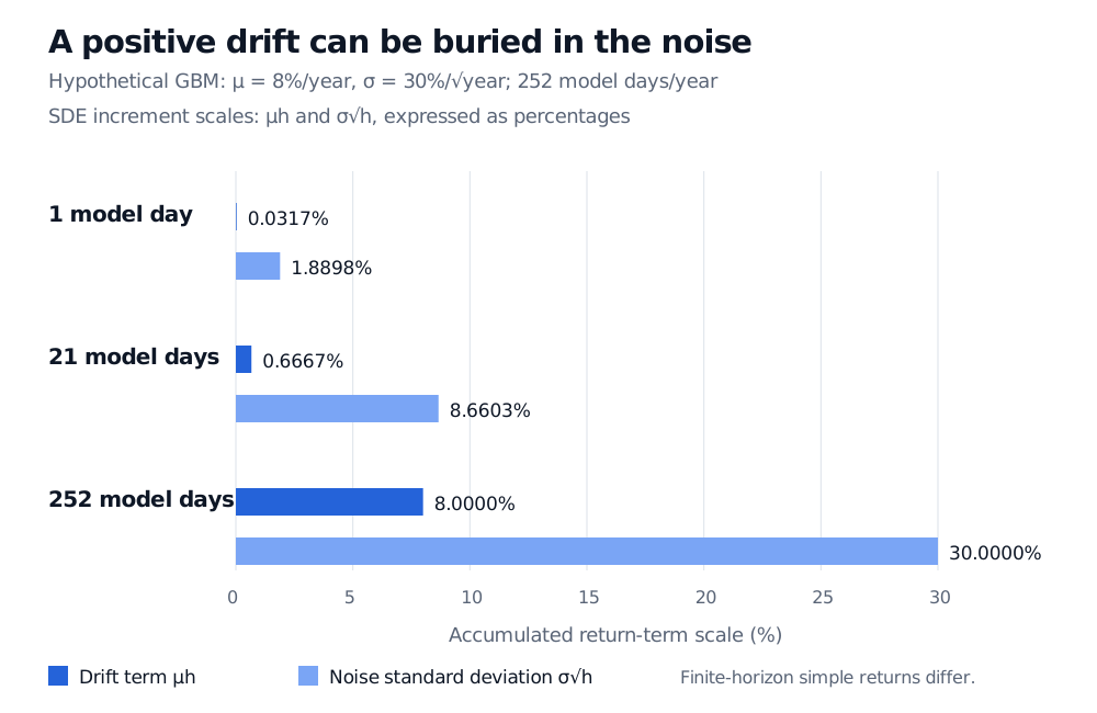
μh=0.0003174603≈0.0317%,σh=0.0188982237≈1.8898%.
The noise standard deviation is about 59.5 times the drift contribution. It is a standard deviation, not a maximum loss or a bound on tomorrow's move. More frequent observations do not turn each individual return into a reliable signal of the drift.
Drift terms for 1, 21 and 252 model days are 0.0317%, 0.6667% and 8%; diffusion standard deviations are 1.8898%, 8.6603% and 30%.
Original hypothetical model comparison: drift terms grow as h, diffusion scales as h. These are SDE increment scales; they are not the exact finite-horizon mean and standard deviation of simple GBM returns. The 252-day clock is a modelling convention, not a calendar identity.
The graph is particularly easy to misread at one year. An 8% instantaneous proportional drift does not mean the exact one-year expected simple return is 8%. In this constant-coefficient geometric Brownian motion model it is
EP[StSt+1−1∣Ft]=e0.08−1≈8.3287%.
The linear expression μh is the local approximation to eμh−1. It is useful precisely because the horizon is small; it should not silently replace the exact finite-horizon expression.
Change the variable, change the drift
The proportional price equation is not an ordinary differential equation for the log price. Applying Itô's lemma gives
dlogSt=(μ−21σ2)dt+σdWt.
For the same stock model,
μ−21σ2=0.08−21(0.30)2=0.035.
The drift of the log price is 3.5% per year, while the instantaneous proportional price drift is 8% per year. The difference is 4.5 percentage points per year. The concavity of the logarithm produces this correction; no new economic return has been introduced.
Consequently, the model's one-year expected log return is 0.035, whereas its expected simple return is approximately 8.3287%. Its median one-year simple return is e0.035−1≈3.5620%. An expected log return, a median simple return and a mean simple return are different summaries. Karl Sigman's GBM notes, §§1 and 1.4 develop this relationship, using μ for the log drift; check a source's notation before transferring its parameters.
This also explains why a positive arithmetic drift need not imply positive log drift: sufficiently large σ2/2 can exceed μ. That is a model statement about growth summaries, not a promise that a particular long-run investment result will occur.
State the probability measure
A drift parameter only has meaning within its probability model. The physical-measure μ above is an assumed expected price-growth rate. Estimating it from market returns introduces uncertainty; stipulating it in a simulation does not establish that markets offer that return.
For risk-neutral valuation, a standard frictionless stock model with continuous dividend yield q instead uses price drift r−q under Q, with continuously compounded risk-free rate r. For a non-dividend-paying stock this becomes r. Changing the measure supports a pricing calculation; it does not assert that investors' physical expected return has become the risk-free rate. Hull, 9th Global Edition, §17.3, equation (17.7), makes the dividend adjustment explicit.
Finally, data drift and model drift in monitoring usually refer to changing distributions, relationships or model behaviour over time. Those meanings are separate from the dt coefficient defined here. A model can have a constant stochastic-calculus drift while its realised observations fluctuate; a dataset can change distribution without that change being a simple shift in this coefficient.
For the derivation behind the price/log-price distinction, the Programme lesson on stochastic processes and Itô's lemma develops the GBM solution in §§3.4–3.5 and the mean calculation in Exercise 3.3. The public page is a preview; the full lesson requires membership.
Sources
John C. Hull, Options, Futures, and Other Derivatives, 9th Global Edition, §§14.2–14.3 for drift and diffusion rates and §17.3 for dividend-paying risk-neutral dynamics.
Karl Sigman, Columbia University, Geometric Brownian motion (2006), §§1 and 1.4: log drift, exponential transformation and price moments. His log-drift notation differs from the proportional-drift notation used here.