Stochastic differential equation: Definition & Examples

A stochastic differential equation (SDE) specifies how a stochastic process evolves through time with random inputs. In finance, it can describe a cash balance, asset price, spread or short rate. The equation supplies a model for possible trajectories and their probabilities; it does not forecast the next realised price.

For a scalar, Brownian-driven model, the usual Itô notation is

dX_t=a(t,X_t)\,dt+b(t,X_t)\,dW_t,\qquad X_0=x_0,

where

W_t

is Brownian motion,

a

is the drift, and

b

is the diffusion coefficient. Together with the initial condition, probability law and information available through time, these ingredients define the modelling problem.

What the differential notation means

The defining statement is an integral equation:

X_t=x_0+\int_0^t a(s,X_s)\,ds +\int_0^t b(s,X_s)\,dW_s.

The first integral accumulates the drift through calendar time. The second is an Itô integral. Its nonanticipating convention uses information available before each Brownian increment; for regular integrands it is obtained as the appropriate limit of left-endpoint sums. The solution is adapted to the chosen filtration, so it cannot use tomorrow's shock today.

Brownian paths have no ordinary time derivative. Consequently, dividing the equation by $dt$ does not produce a conventional differential equation with an ordinary random slope $dW_t/dt$ . Nor can the stochastic integral silently be replaced by a Stratonovich integral: when diffusion depends on the state, changing conventions generally requires a drift correction to describe the same process.

Even when $a(t,x)$ is a known deterministic function, $a(t,X_t)$ can be random because $X_t$ is random. “Drift” describes the local conditional direction of movement, rather than a guaranteed deterministic trajectory.

A cash-balance model you can calculate exactly

Suppose a synthetic cash balance, measured in USD, follows

dX_t=2\,dt+3\,dW_t,\qquad X_0=100,

with time measured in years. This additive model is arithmetic Brownian motion. The coefficient 2 has units USD/year. Because Brownian increments have standard deviation $\sqrt{h}$ over $h$ years, the coefficient 3 has units USD/ $\sqrt{\text{year}}$ . The resulting variance rate is 9 USD²/year. These units prevent a common simulation mistake: noise scales with the square root of elapsed time, while the drift contribution scales with elapsed time itself.

The coefficients are constant, so integrating gives the exact transition

X_{t+h}=X_t+2h+3\sqrt{h}\,Z, \qquad Z\sim\mathcal{N}(0,1),

where $Z$ is independent of information at $t$ . At $t=0$ , take $h=0.25$ year and specify a shock $Z=1$ . Then

\begin{aligned} \Delta W&=\sqrt{0.25}\times1=0.5,\\ X_{0.25}&=100+2(0.25)+3(0.5)=102. \end{aligned}

Before observing the shock, the quarter-year endpoint has mean USD 100.50 and standard deviation USD 1.50:

X_{0.25}\sim\mathcal{N}(100.5,\,2.25).

The second parameter here is the variance in USD². USD 102 is one selected endpoint, one standard deviation above the mean; it is not the expected balance.

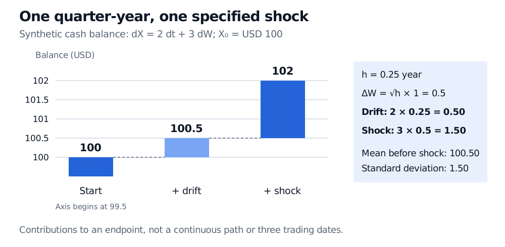
Synthetic cash balance starts at USD 100, gains USD 0.50 from drift and USD 1.50 from the specified shock, ending at USD 102. Before observing the shock, the mean is USD 100.50 and standard deviation USD 1.50.

Constant-coefficient additive model over 0.25 year, with the specified standard-normal shock $Z=1$ . Bars show contributions to one endpoint; the level axis begins at USD 99.50.

This can be a simple model for cash that may move into borrowing. It would be unsuitable for an asset price that must stay positive: its normal transition distribution allows negative balances. That is a property of the assumed model, not a numerical failure.

The SDE and its simulation scheme are different objects

A general SDE rarely integrates as simply. The Euler–Maruyama method freezes the coefficients at the start of each step:

\widehat X_{n+1}=\widehat X_n +a(t_n,\widehat X_n)h +b(t_n,\widehat X_n)\sqrt{h}\,Z_n,

with independent standard-normal

Z_n

. Hats mark numerical approximations. For the constant-coefficient cash model, this happens to give the exact values at the grid points. Additive noise alone does not make Euler exact: the drift may still vary during a step, as it does in the Ornstein–Uhlenbeck process.

Now use geometric Brownian motion:

dS_t=\mu S_t\,dt+\sigma S_t\,dW_t.

Set $S_0=100$ , $\mu=0.08$ per year, $\sigma=0.20$ per square-root year, and use the same $h=0.25$ , $Z=1$ . Euler gives

\widehat S_1=100\left(1+0.08(0.25)+0.20(0.5)\right)=112.

The exact GBM transition instead gives

S_{0.25}=100\exp\left[\left(0.08-\frac{0.20^2}{2}\right)0.25 +0.20(0.5)\right] \approx112.1873.

The difference is about USD 0.1873 for this shock and step. Both calculations use the same Brownian increment; the discrepancy comes from the approximation rule. It is not evidence of a different shock, an estimated market error or a universal direction of pricing bias.

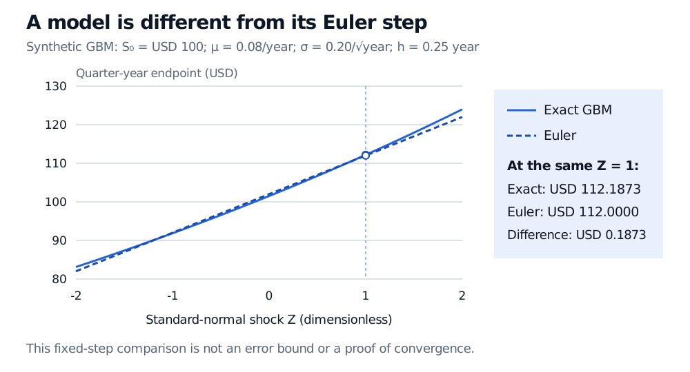
Exact GBM and Euler endpoint values plotted against the same standard-normal shock from minus 2 to 2. At shock 1, Euler gives USD 112 and exact GBM gives USD 112.1873.

Original analytic comparison for a synthetic quarter-year GBM model. The horizontal axis varies the shock, not time. The exact transition is exponential; Euler uses a straight-line approximation.

An exact transition samples the model correctly at the chosen dates. It still does not reveal every movement between those dates. For a barrier payoff, missing an intervening crossing can matter even when the endpoint samples are exact.

Before trusting the model

Writing an SDE does not establish that a solution exists or is unique. A standard sufficient result uses coefficients that are globally Lipschitz in the state, with at most linear growth, on a finite horizon, plus suitable measurability and an initial condition with finite second moment. It yields a unique adapted strong solution driven by the given Brownian motion. These conditions are sufficient rather than necessary; square-root diffusions require more specialised analysis.

Existence of a solution also does not guarantee that a chosen numerical scheme behaves well. Convergence, stability, boundary behaviour and the payoff being estimated need their own checks. For simulation comparisons, use common Brownian increments so a change of random input does not obscure discretisation error.

Finally, the probability measure belongs to the specification. A drift chosen for real-world scenario generation need not equal the drift under a risk-neutral measure. A syntactically correct SDE, or an accurate solver, cannot by itself justify a pricing assumption or establish that a model fits financial data.

For the financial model sequence, the Stochastic Processes, Brownian Motion and Itô's Lemma lesson develops ABM, GBM, OU and the log transformation behind the exact GBM step. Its public preview is open; the full lesson requires membership.

Sources

John C. Hull, Options, Futures, and Other Derivatives, 9th Global Edition, Chapter 14 §§14.2–14.3 and §14.6: generalised Wiener processes, state-dependent coefficients, stock-price dynamics and Itô's lemma.
Desmond J. Higham, “An Algorithmic Introduction to Numerical Simulation of Stochastic Differential Equations,” SIAM Review 43(3), 2001, §§3–5 and §7: integral conventions, Euler–Maruyama, exact GBM comparison, convergence and stability.
MIT OpenCourseWare, 18.S096, Fall 2013, Lecture 21, §1, Theorem 1.1 and §1.1: sufficient existence and uniqueness conditions and the GBM solution.

What the differential notation means

A cash-balance model you can calculate exactly

The SDE and its simulation scheme are different objects

Before trusting the model

Sources

Related terms

Brownian motion

Drift

Filtration

Geometric Brownian motion

Itô integral

Ornstein-Uhlenbeck process

Stochastic process