The OU process combines mean reversion with Gaussian shocks. Derive its exact transition, distinguish conditional and stationary laws, and connect half-life to AR(1) sampling.
Ornstein-Uhlenbeck process
An Ornstein-Uhlenbeck process, or OU process, is a continuous-time model in which a variable is pulled toward a fixed level while receiving additive random shocks. It is a standard model for a signed spread, a factor residual or a Gaussian short rate. Its appeal is practical: both the forecast distribution and an exact simulation step are available in closed form.
The restoring force acts on the conditional mean. It does not require the next observed movement to be toward equilibrium, keep the process inside a band, or guarantee a profitable convergence trade.
Here Wt is standard Brownian motion, θ is the long-run level, κ is the speed of mean reversion, and σ is the diffusion coefficient. With time measured in years and X in spread points, their units are respectively points, per year and points per square-root year. The diffusion coefficient is not the long-run standard deviation.
Above θ, the drift is negative; below it, positive. At θ, the drift vanishes but the shocks remain. This is an equilibrium level for the distribution, rather than a place where the process stops. A centered OU process uses θ=0; subtracting θ from a nonzero-mean model gives that centered form.
To see why the model is tractable, set Yt=Xt−θ and multiply by eκt. The time derivative of the multiplying factor cancels the restoring drift:
d(eκtYt)=σeκtdWt.
Consequently, conditional on the observed value Xt=x, the future level is
Xt+h=θ+(x−θ)e−κh+σ∫tt+he−κ(t+h−s)dWs.
The last term is an Itô integral with a deterministic integrand. It is a zero-mean normal shock, independent of information available at t. Integrating its squared coefficient gives the variance. This integrating-factor argument is developed for the centered process in Jonathan Mattingly's Duke notes.
Consider a synthetic spread measured in points. Suppose its stipulated parameters are κ=2 per year, θ=3 points and σ=1.2 points per square-root year. Today the spread is 9 points. These are illustrative assumptions, rather than estimates from market data.
The conditional standard deviation is about 0.557924 points. The forecast has moved toward 3, yet it remains well above 3 because the current displacement still matters. Replacing the conditional mean with θ would discard information we have just observed.
The expected displacement halves after
h1/2=κln2.
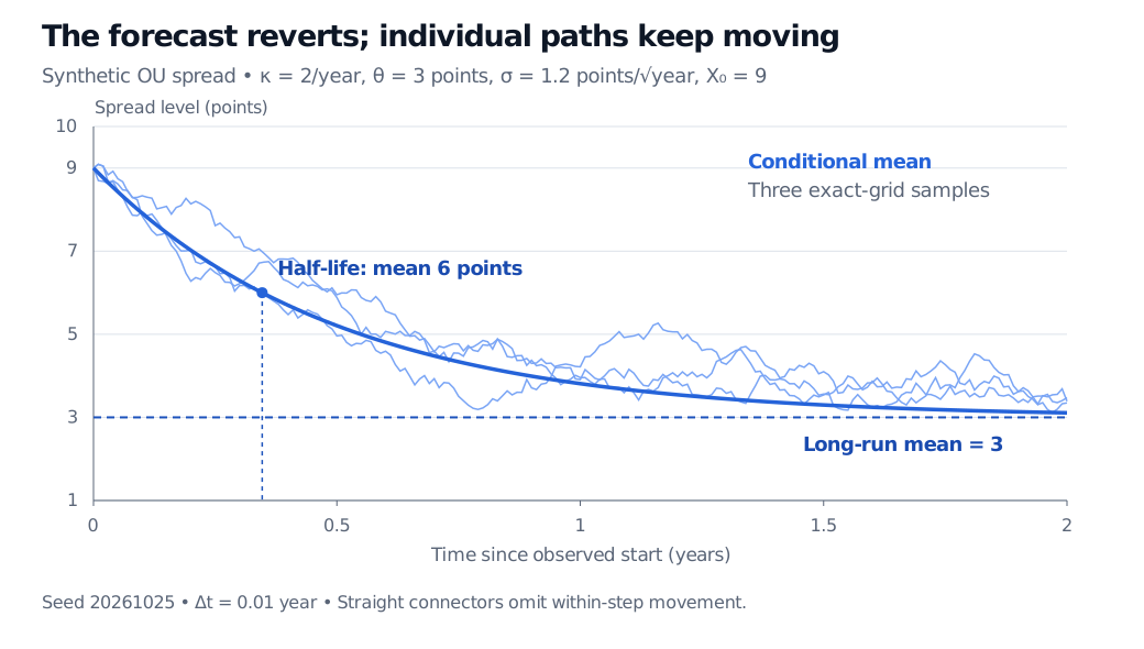
Here that is 0.346574 years: the expected level falls from 9 to 6, halving its initial six-point gap above 3. This is a half-life of the expected signed displacement. It is neither an expected first-passage time to 6 nor a deadline by which a sample path must cross that level. Hitting-time questions require a separate calculation.
Synthetic OU spread starts at 9 points and has long-run mean 3. The conditional mean reaches 6 after 0.346574 years. Three seeded exact-grid paths fluctuate around the mean forecast.
Original synthetic model. Three paths use seed 20261025 and exact transitions every 0.01 year. Straight connectors do not show all movement between observations.
What “stationary” adds
As the forecast horizon grows, the conditional mean approaches θ and the conditional variance approaches σ2/(2κ). The invariant, or stationary, distribution is
N(θ,2κσ2).
For the example, it has mean 3 points, variance 0.36 points squared and standard deviation 0.6 points. Andrey Sarantsev's notes give this nonzero-mean OU model and its invariant normal law in §§19.3–19.5.
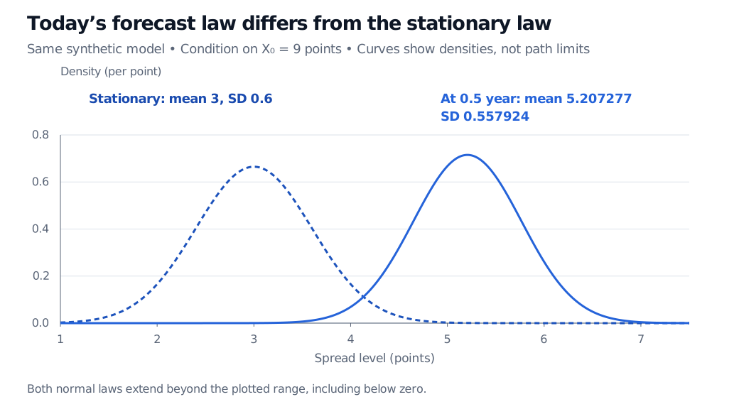
Starting at a known 9 does not make the process stationary from time zero. Its time-zero law is concentrated at 9; its subsequent distributions change. To construct the stationary process from the start, draw the initial state from the invariant normal law, independently of future Brownian increments. The future marginal distribution then remains the same, although successive levels remain dependent. In that stationary regime,
Corr(Xt,Xt+h)=e−κh.
Two normal density curves for the same synthetic OU model. At half a year conditional on a starting level of 9, mean is 5.207277 and standard deviation 0.557924. The stationary curve has mean 3 and standard deviation 0.6. Both have unbounded support.
Original model densities. A fixed initial state produces a changing conditional law; the stationary law describes equilibrium initialization or the long-horizon limit.
A bounded variance is not a bounded state space. With positive σ and a positive horizon, the normal transition density assigns positive probability to levels below zero and beyond any finite band. This suits signed residuals but requires care for quantities that must remain nonnegative. Mean reversion also does not mean individual paths settle permanently at θ.
Exact sampling, and the AR(1) connection
At equally spaced observation times, the OU process satisfies the exact recursion
This is an AR(1) model with an intercept. It samples the continuous-time model exactly at the grid points, as in the transition exercise in Jun Yan's statistical-computing notes, §5.3.3. Omitting the intercept is valid for the centered state X−θ, but changes a general nonzero-mean model. A fitted AR coefficient must lie strictly between zero and one to map to this mean-reverting scalar OU model with finite positive κ.
An Euler step instead replaces ϕ with 1−κΔ and the innovation variance with σ2Δ. That is an approximation. For our example, one Euler step of half a year gives mean 3 and variance 0.72, versus the exact 5.207277 and 0.311279. A coarse step can substantially distort both the speed and uncertainty of reversion; this model already provides a simple exact alternative.
In finance, fitting OU dynamics is still a modelling decision. The long-run level and speed may change, shocks may have heavier tails, and a residual may contain estimation error. Historical mean reversion supplies a conditional statistical forecast, not a guaranteed trade: costs, borrow, execution and exposure to model failure still matter. A short-rate model used for pricing also needs parameters under the appropriate pricing measure; historical residual estimates do not automatically supply them.
Ioannis Karatzas and Steven E. Shreve, Brownian Motion and Stochastic Calculus, first edition, 1988, Chapter 5, §6A, Example 6.8, p. 358: scalar OU solution, moments and stationary covariance.
Gregory F. Lawler, Stochastic Calculus: An Introduction with Applications, revision of 15 February 2023, Chapter 4, Exercise 4.1: linear OU SDE and exit-time formulation.