Mean reversion: Definition & Examples

Mean reversion is a model property in which deviations from a reference level tend to diminish in the conditional forecast. When the state is above that level, its expected change points down; when it is below, its expected change points up. The next realised move can still go either way.

For a quant researcher, the distinction matters immediately: a spread can have a forecast of narrowing while the position betting on that narrowing loses money. Mean reversion describes the dynamics of a specified variable under specified assumptions. It does not establish fair value, a return deadline or a profitable trading rule.

A spread with a restoring pull

Suppose $X_t$ is a hypothetical, tradable portfolio spread measured in USD per fixed unit of the portfolio, observed once per day. Assume its daily dynamics follow an autoregressive model of order one:

X_{t+1}=\mu+\phi(X_t-\mu)+\varepsilon_{t+1}, \qquad 0<\phi<1.

Here $\mu$ is the reference level and $\phi$ is persistence: the fraction of today's deviation retained in tomorrow's forecast. Assume independent, identically distributed Gaussian innovations with mean zero and standard deviation $\sigma_\varepsilon$ , independent of the observed history. Parameters are known and constant throughout this example.

Taking the conditional expectation given information available at day

t

gives

\mathbb{E}[X_{t+1}-X_t\mid X_t] =(1-\phi)(\mu-X_t).

This equation identifies the restoring pull. It is not the statement that tomorrow's spread must be closer to $\mu$ : a new innovation can overpower the expected change.

Set $\mu=2$ , $\phi=0.8$ , $\sigma_\varepsilon=0.6$ and today's spread $X_0=6$ , all spread amounts in USD. Then

\mathbb{E}[X_h\mid X_0=6]=2+4(0.8)^h.

Forecast horizon	Conditional mean (USD)	Gap from reference level (USD)
Today	6.0000	4.0000
1 day	5.2000	3.2000
2 days	4.5600	2.5600
3 days	4.0480	2.0480
4 days	3.6384	1.6384
10 days	2.4295	0.4295

The one-day expected change is

-0.8

dollars. If the same model is written

X_{t+1}=c+\phi X_t+\varepsilon_{t+1}

, its intercept is

c=(1-\phi)\mu=0.4

, not the long-run mean 2. Confusing the intercept with the mean changes the target of every forecast.

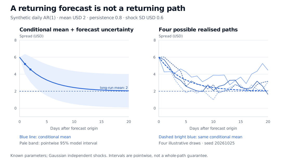
Synthetic daily AR(1) spread starting at USD 6 with long-run mean USD 2, persistence 0.8 and innovation standard deviation USD 0.6. The one- and two-day forecasts are USD 5.20 and USD 4.56. A pointwise 95 percent forecast band widens while four seeded possible paths fluctuate and can move away from the mean.

Original model illustration: known parameters, independent Gaussian innovations, daily observations and four draws using seed 20261025. The pale band gives a 95% interval separately at each horizon; it does not contain an entire future path with 95% probability. Straight connectors join observations.

Half-life measures forecast decay, not waiting time

For positive persistence, the forecast deviation shrinks by half when

\phi^h=1/2

. Its half-life is

h_{1/2}=\frac{\log(1/2)}{\log\phi} =\frac{\log(1/2)}{\log(0.8)} \approx3.1063\text{ days}.

The model is observed at integer days. The fractional value summarises the geometric decay rate; the first integer-day forecast with a gap no larger than USD 2 is day 4. Day 3's gap is still USD 2.048.

That half-life is neither the expected first-passage time to the mean nor the median time a trade takes to close. A first-passage question needs a boundary, a monitoring rule and a distribution of entire future paths. For a discretely observed Gaussian spread, landing exactly on the reference level at any particular future observation has probability zero; crossing it or entering a tolerance band is a different event. A realised path might cross early, move away first, or remain above it throughout a chosen holding period.

The mean settles; uncertainty remains

Forecast convergence does not make the future state deterministic. With the fixed initial value and known parameters above,

\text{Var}(X_h\mid X_0=6) =\sigma_\varepsilon^2\sum_{j=0}^{h-1}\phi^{2j} =\frac{\sigma_\varepsilon^2(1-\phi^{2h})}{1-\phi^2}.

The conditional variance is $0.36$ USD squared after one day and $0.5904$ USD squared after two. At long horizons it approaches

\frac{0.6^2}{1-0.8^2}=1\text{ USD}^2,

so uncertainty approaches a standard deviation of USD 1 rather than zero. The limiting Gaussian distribution is centred at 2 with variance 1. A process started in that distribution is stationary; our ensemble started at the fixed value 6 is not initially stationary, even though it approaches the same distribution.

A finite stationary variance is not a hard range. Gaussian innovations give the spread unbounded support. Mean reversion can coexist with rare, large deviations, and a finite simulation's highest and lowest points do not become model bounds.

The sign of persistence also matters. With

-1<\phi<0

, forecast deviations alternate sides while shrinking in magnitude. With

\phi=1

, this model becomes a random walk: the restoring pull disappears and the current level remains the forecast at every horizon. At

\phi=0

, the next forecast immediately equals

\mu

. The positive-persistence half-life formula above should not be applied indiscriminately to these cases.

What the model leaves for research

A chart that repeatedly turns around is not evidence enough to establish mean reversion. Short random-walk samples can appear anchored; a structural break can make a previously stable mean irrelevant. Estimation must distinguish a persistent stationary model from a unit root, assess residual dependence and test forecasts on later observations. Near $\phi=1$ , small estimation changes can greatly change the implied decay time. The calculations above omit parameter uncertainty.

Specify what should revert. Individual asset prices need not revert merely because a portfolio spread does; cointegration concerns stationary combinations of suitable nonstationary series. Reversion of volatility, a short rate and a price residual are different empirical hypotheses. In continuous time, an Ornstein–Uhlenbeck process provides a familiar model with a restoring drift, but choosing that model still requires evidence.

Even if the spread forecast is correct, a mean-reversion strategy must translate the spread into actual holdings. Financing, borrow availability, execution costs and losses before convergence affect the result. A model fitted under a pricing measure also need not describe real-world expected trading gains. The expected narrowing of a spread and a guaranteed net profit are separate claims.

For the forecasting machinery, the AR, MA, and ARMA lesson develops persistence, stationarity conditions, residual diagnostics and multi-step forecast variance. The public page is a preview; the full lesson requires membership.

Sources

Chris Brooks, Introductory Econometrics for Finance, 2nd edition, Cambridge University Press, 2008, §§5.4.1–5.4.2 and Example 5.4 (autoregressive stationarity, mean and variance), and §5.11.7 (recursive forecasts). The numerical spread and figure are original.
Liberty Hamilton, Lecture 16 Notes — AR Models, UC Berkeley STAT 153/248, Spring 2026, sections “AR(1) process” and “Properties of the stationary AR(1) model”: persistence regimes, stationary variance and geometric autocorrelation decay.

A spread with a restoring pull

Half-life measures forecast decay, not waiting time

The mean settles; uncertainty remains

What the model leaves for research

Sources

Related terms

Cointegration

Conditional expectation

Ornstein-Uhlenbeck process

Random walk

Stationarity