Distinguish strict and weak stationarity, stationary increments and ergodicity using iid levels, a deterministic trend and a random walk.
Stationarity
Stationarity means that specified probabilistic features of a time series remain unchanged when its observation times shift together. It is a property of the generating process. For a quant estimating a spread's usual level or a return's variance, the practical question is whether observations from different dates describe the same statistical object.
Which features must remain unchanged depends on the definition. A stationary process need not be independent, predictable, bounded, or profitable to trade.
The distribution, or just its first two moments?
Strict stationarity requires every finite collection of observations to have the same joint distribution after a common time shift:
(Xt1,…,Xtk)=d(Xt1+h,…,Xtk+h).
This holds for every collection of times and every shift h for which both collections are defined. Equal single-date distributions alone are insufficient: the dependence between dates must also survive the shift.
Weak stationarity, also called covariance stationarity, requires finite second moments and
E[Xt]=μ,Var(Xt)=γ(0)<∞,Cov(Xt,Xt+h)=γ(h).
The covariance may depend on the lag h, but not on the starting date t. Constant variance is the lag-zero case of the same requirement. Weak stationarity does not require zero autocovariance.
The moment qualification matters. Strict stationarity implies weak stationarity when second moments are finite; iid Cauchy observations are strictly stationary but have no finite variance. Conversely, independent observations alternating between standard-normal and equally likely −1,+1 distributions have constant mean zero, variance one and zero nonzero-lag covariance. They are weakly stationary, but their alternating marginal laws prevent strict stationarity. For a jointly Gaussian process, means and covariances determine every finite joint law, so weak stationarity does imply strict stationarity.
Three models to test the definition
Imagine testing whether a model output could serve as a stable spread benchmark. Use equally spaced observation times and dimensionless states; these are synthetic models, not actual asset prices. Let the shocks εt be independent and identically distributed N(0,1) variables.
Model, for t≥1
Population mean
Population variance
Conclusion
IID levels: Xt=εt
0
1
Strictly and weakly stationary
Deterministic trend: Tt=100+t+εt
100+t
1
Nonstationary mean
Random walk: Yt=∑j=1tεj, Y0=0
0
t
Nonstationary variance
The iid model has γ(0)=1 and γ(h)=0 for every nonzero lag. It is stationary even though past observations provide no prediction of the next independent shock.
The trend model's mean rises from 101 at t=1 to 110 at t=10. Its variance stays at one, so checking variance alone would miss its nonstationarity.
The random walk has a constant mean, but independence of the innovations gives
Var(Yt)=j=1∑tVar(εj)=t.
Its variance is one at t=1 and ten at t=10. Moreover,
Cov(Ys,Yt)=min(s,t).
The pairs (Y2,Y5) and (Y7,Y10) both have lag three, yet their covariances are two and seven. The covariance depends on the dates, not just their separation. A flat expected level therefore does not establish stationarity.
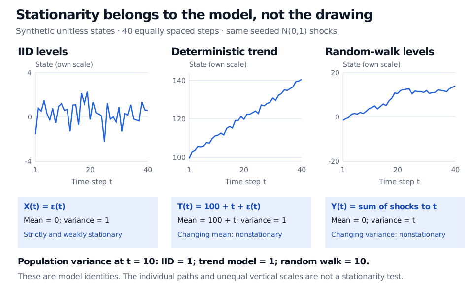
Three synthetic paths with shared iid standard-normal shocks: iid levels have mean zero and variance 1; a 100 plus time trend has changing mean and variance 1; a random walk has mean zero and variance t, reaching population variance 10 at time 10. The three panels use different vertical scales.
Original seeded model illustration, dimensionless states and equally spaced time steps. Each panel has its own vertical scale. The stated means and variances are population identities, not estimates from these 40 observations.
Stationary changes can coexist with nonstationary levels
A process has stationary increments when the distribution of a change over a fixed-length interval does not depend on when that interval begins. This concerns changes, rather than levels.
For the random walk above,
ΔYt=Yt−Yt−1=εt,Yt+h−Yt∼N(0,h)
for positive integer h. Every three-step increment has variance three, whether it starts at step two or step seven. The levels remain nonstationary. Stationary increments also do not, by themselves, imply independent increments; this walk has both because of its stipulated iid shocks.
Differencing works here because of the model. It does not automatically remove changing volatility, breaks, or every form of trend. For Tt, subtracting the known deterministic component 100+t recovers the stationary shock. If a financial series is a log price, its log difference is a log return, but that algebra alone says nothing about whether the return process is stationary. The transformed series needs its own justification.
Stationarity is not ergodicity
Ergodicity supplies an additional connection between time averages along a history and expectations across possible histories. For a stationary ergodic process with an integrable state, the time average converges almost surely to its population mean. Convergence of the mean alone is a narrower property than full ergodicity.
Draw one random sign Z, equally likely to be −1 or +1, and set At=Z for every date. Every shifted joint distribution is identical, so this process is strictly and weakly stationary. Its population mean is zero and its variance is one. But
n1t=1∑nAt=Z
for every sample length. One history stays at +1 or −1 forever; its average never reaches the ensemble mean zero. More observations do not reveal a new draw of Z.
That distinction matters when treating one market history as a source of long-run estimates. Stationarity by itself does not justify replacing population moments with historical sample moments.
What a trading researcher can conclude
A short plot cannot establish stationarity, and a series that looks quiet can still contain a stochastic trend. Unit-root and stationarity tests provide evidence under specific null hypotheses, lag choices and deterministic terms; they do not certify permanent stability. Changing market regimes can invalidate a previously useful model.
Stationarity also does not guarantee mean reversion at a tradable speed, a finite holding period, or a cap on losses. Even the stationary iid Gaussian model above has unbounded support. Cointegration concerns a stationary combination of nonstationary series under a model; whether that combination offers a usable strategy still depends on forecasting, execution and costs.
The Stationarity and Unit Roots lesson develops the testing and model-selection questions. Its public page is a preview; the full lesson requires membership.
Sources
William H. Greene, Econometric Analysis, 5th edition, §12.4.1, Definitions 12.1–12.2 and Theorem 12.1: stationarity and the time-average estimation argument.