The ratio is exact; the percentage interpretation is approximate
Write the ordinary proportional change, or simple return, as . Then
The approximation follows from near zero. It is less reliable for large moves. A log difference is not the logarithm of the ordinary difference: would fail even for a perfectly valid decline between two positive observations.
A round trip in percentages is not a round trip in wealth
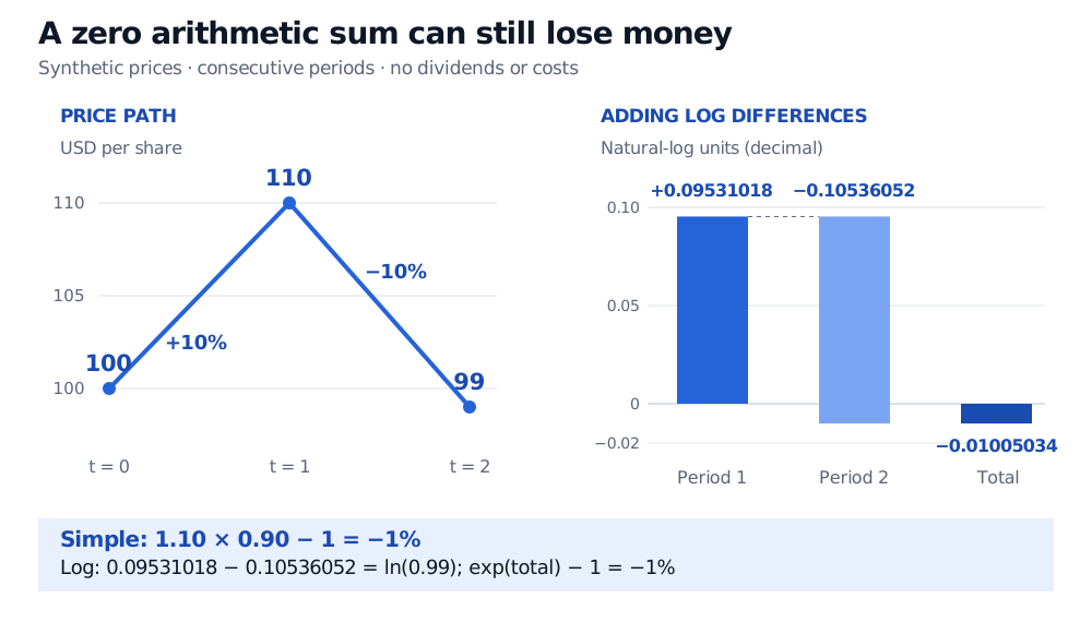
Suppose a hypothetical share closes at USD 100, USD 110 and USD 99 over two consecutive periods. There are no dividends, splits or costs.
| Interval | Simple return | Log difference, decimal |
|---|---|---|
| 100 to 110 | +10% | 0.09531018 |
| 110 to 99 | −10% | −0.10536052 |
| Full interval, 100 to 99 | −1% | −0.01005034 |
The loss is applied to 110, a larger base than the initial 100. Adding gives zero, but the full-period simple return is
Log differences add exactly across consecutive observations:
Here the unrounded sum is . Exponentiating that sum and subtracting one recovers the −1% simple return. The identity needs no assumption of independent or normally distributed returns.
Units disappear only when they are consistent
Multiplying every observation by the same positive constant leaves the log difference unchanged:
Prices quoted consistently in cents therefore produce the same log differences as prices quoted consistently in dollars. Formally, logging relative to a fixed positive reference level also avoids taking a logarithm of a dimensional quantity; the reference cancels on differencing.
A time-varying conversion does not cancel. Translating foreign-currency prices into domestic currency adds the exchange-rate log change to the local-price log change. That is a different investment exposure. Using base-10 logarithms also changes the numerical scale: divide the natural-log difference by to obtain the base-10 difference.
A log difference describes the entire observation interval. Divide by elapsed years to report an average continuously compounded annual rate. Across irregular observation gaps, the same log difference can represent very different annual rates. Summing observed consecutive log differences still yields the endpoint change, but a missing date does not become an observed zero-return day.
Check what the observations represent
For series that can cross zero—such as profit, a spread or some futures prices—choose a transformation suited to the economic question. Adding an arbitrary constant before logging changes the measured proportional change and makes it depend on the chosen offset and units. It does not preserve the original log-return interpretation. Taking absolute values discards the sign.
Prices also need a consistent economic basis:
- Splits: in an otherwise unchanged two-for-one split, a USD 100 share becomes two USD 50 shares. Logging the unadjusted quotes reports , despite unchanged position value. Use a consistently split-adjusted series. This is the share-count mechanism described by Investor.gov.
- Dividends: a price log difference alone measures price return. For example, a USD 100 share ending at USD 98 while paying USD 2 cash at the interval end has a −2% price return but a zero total return before costs. To study total return, use a documented reinvested total-return series or explicitly account for distributions. Check the provider's adjustment and reinvestment conventions before treating an “adjusted close” as that series.
Sources
- John C. Hull, Options, Futures, and Other Derivatives, 9th Global Edition, §15.2, equation (15.6), and §15.3: continuously compounded rates and the distinction from arithmetic returns.
- Rob J. Hyndman and George Athanasopoulos, Forecasting: Principles and Practice, 3rd edition, §3.1, “Mathematical transformations”: logarithmic transformations, scale and domain.
- U.S. Securities and Exchange Commission, Investor.gov: Stock Split: share-count and price changes under a split.