Measure return dispersion, calculate a daily sample estimate, and distinguish annualisation, historical volatility, conditional forecasts and implied volatility.
Volatility
Volatility is the scale of variation in an asset's returns, usually measured by their standard deviation over a stated interval. It measures dispersion around an expected or estimated mean. A volatility figure needs a return definition, observation frequency and horizon: “20% volatility” alone is incomplete.
For a trader, the distinction is practical. A position can have a small average daily return while experiencing large gains and losses. Its volatility describes the size of those fluctuations; it does not tell you which sign comes next. It is one input to position sizing, portfolio risk and option pricing, rather than a complete description of any of them.
Three days, with no average move
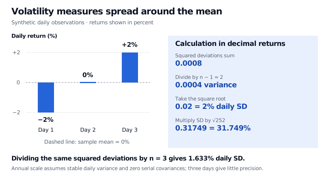
Suppose an analyst has three synthetic daily log returns, expressed as decimals:
r1=−0.02,r2=0,r3=0.02.
These are continuously compounded returns, rt=log(Pt/Pt−1), for positive prices with no intervening cash flows. Their sample mean is zero. That does not make the investment riskless: two of the observations are two percentage points away from the mean.
A common centred historical estimator, for n≥2 observations, is
rˉ=n1t=1∑nrt,s2=n−11t=1∑n(rt−rˉ)2,s=s2.
Here the squared deviations sum to 0.0008, so
s2=20.0008=0.0004,s=0.02=2%.
The daily variance is 0.0004 in squared decimal-return units; the daily volatility is 0.02 in decimal-return units. If returns are entered as percentage-point numbers −2, 0 and 2, the same calculation gives variance 4 in squared percentage points and standard deviation 2 percentage points. Squaring and taking a square root changes the units: variance 0.0004 is not “0.04% volatility.”
Three synthetic daily log returns of minus 2%, zero and plus 2% have mean zero, sample variance 0.0004 in squared decimal-return units and sample standard deviation 2%. Annualising at 252 observations gives 31.749%. Dividing squared deviations by three instead gives daily standard deviation 1.633%.
Original synthetic example. Daily log-return observations, centred sample estimator with divisor n − 1. The annual scale assumes stable daily variance and zero serial covariances.
The divisor matters. Using n=3 instead gives 0.0008/3≈0.0163299, or 1.633%. That is the population standard deviation of the three-point empirical distribution with equal weights; it is also a different estimation convention from the sample formula above. Neither software's default should be assumed silently. Under iid sampling with finite variance, the n−1 correction makes the sample variance unbiased; taking its square root does not generally produce an unbiased standard-deviation estimator.
What annualisation assumes
With 252 daily observations per year, the usual annualised estimate is
σann=s252=0.02252≈0.3174902=31.749%.
Variance scales by 252, giving 252s2=0.1008; standard deviation scales by its square root. Annualising three observations does not create a year's worth of evidence. This sample is deliberately too short to support a precise risk forecast.
The mathematical basis is the variance of a sum:
Var(t=1∑mrt)=t=1∑mVar(rt)+2i<j∑Cov(ri,rj).
Common finite daily variance and zero serial covariances give variance mσd2 and volatility mσd. Iid returns with finite variance are sufficient; normality is unnecessary for this identity. Log returns add over time, so the sum represents the multiperiod log return. Simple returns compound instead, and the same square-root rule is not an exact identity for their compounded return.
Applying this scale to the future additionally assumes that the estimated daily variance remains relevant. Changing variance or nonzero serial covariances can invalidate that extrapolation. Volatility clustering concerns dependence in return magnitudes; it does not by itself imply nonzero covariance between signed returns. The observation clock also matters: a 252-trading-day convention cannot be swapped for calendar days without changing the model and inputs.
Historical, conditional and implied answer different questions
The volatility input that makes a specified option-pricing model match an observed option price
A price-implied model parameter for a particular contract and set of conventions
“Realised volatility” can also denote measures constructed from sums of squared intraday returns. Those need not use the centred sample formula above; compare the actual definitions before comparing the numbers.
An implied figure is forward-looking market-price information, but it is not a direct observation of future volatility or an unbiased physical-world forecast. It depends on the pricing model, contract terms and prices, which reflect compensation for risk as well as expectations. Entering a chosen volatility into an option calculator produces a scenario price; it does not measure historical volatility or discover tomorrow's uncertainty.
Read the number alongside the risk
Volatility treats deviations above and below the mean symmetrically. Reflecting every return's sign leaves its standard deviation unchanged. It therefore cannot substitute for a downside-loss measure, maximum drawdown, or a description of tail outcomes. A one-standard-deviation band is not a hard limit on losses, and a coverage probability requires a distributional assumption.
Before comparing two volatility estimates, align the return basis, adjustments for splits and cash distributions, timestamps, lookback window, centering, divisor and annualisation convention. Different inputs can explain a difference without either calculation being arithmetically wrong. Stale prices and sparse observations can also hide movements between recorded marks.
For the next step, Financial Return Characteristics develops simple versus log returns, tails and volatility clustering. Its public page is a preview; the complete lesson requires membership.
Sources
John C. Hull, Options, Futures, and Other Derivatives, 9th Global Edition, §15.4 (historical estimation and time units), §15.11 (implied volatility), and §23.1 (centering, divisors and weighting conventions).