Separate option contract, pricing model and calculation method; compare analytical, tree, Monte Carlo, PDE and Fourier approaches with an independently checked same-model benchmark.
Option pricing assigns a value today to an option's future rights and payments, using its contract terms, market inputs, and valuation assumptions. The result is a model value for the premium. It is different from the payoff received at exercise or expiry, and from the buyer's eventual profit.
The first decision is what to value. The next is which model describes the risks and their prices. Only then does it make sense to choose a formula, tree, simulation, differential-equation solver, or transform method.
That ordering prevents a common mistake: treating “Black–Scholes,” “Monte Carlo,” and “Heston” as interchangeable entries on a list of pricing models. Some names identify dynamics; others identify ways to calculate with those dynamics.
Freeze the contract before choosing the calculation
Owen is checking two implementations of a pricing engine. One returns 10.45 and the other 10.52. Before deciding which is better, he writes down the problem they are supposed to solve.
Layer
Owen's illustrative specification
Contract
European call, covering one underlying unit; strike 100 USD; expiry exactly one year from valuation; no barriers or averaging
Exercise and payment
Exercise only at expiry; terminal payoff (ST−100)+, paid then
Black–Scholes–Merton dynamics, with constant volatility, rate and yield; frictionless trading and financing assumptions
Valuation
Risk-neutral valuation under the specified model; no taxes, fees or funding adjustments
For this fixed-rate European terminal payoff, the calculation targets
V0=e−rTEQ[(ST−K)+].
The risk-neutral measure Q belongs to the pricing specification. It is not Owen's forecast of the stock's actual return. Other contracts require their own cash flows and exercise decisions: an American option, for example, includes the right to exercise before expiry.
The analytical benchmark for Owen's call is 10.45058 USD per underlying unit. If the stock eventually finishes at 120, the payoff is 20. The buyer's simple expiry profit is approximately 20−10.45058=9.54942, ignoring financing and fees. None of those three quantities is a substitute for the others.
One model can support several methods
The analytical formula and a suitably refined numerical approximation should agree when they solve the same contract under the same model and conventions. They need not give identical numbers on a finite grid or with a finite random sample.
Method
Where it helps
What needs attention
Analytical Black–Scholes formula
Extremely fast European vanilla benchmark under the constant-volatility model
Its closed-form contract and model assumptions must fit the problem; it does not add early exercise or discrete cash dividends automatically
Binomial tree
Transparent backward valuation; early exercise can be compared with continuation at each permitted node
Step size, parameterization and exercise dates affect accuracy; extra risk factors or path information enlarge the state space
Flexible sampling for many risk factors and path-dependent cash flows
Sampling error, possible time-discretization bias, and payoff monitoring; a simple terminal-payoff average does not solve American exercise
PDE / finite differences
Low-dimensional state grids, prices and sensitivities across states; exercise constraints or barriers can be incorporated
Spatial and time grids, boundary conditions and stability; additional dimensions become expensive, and payoff kinks can disturb numerical sensitivities
Fourier methods
Efficient European pricing, often across many strikes, when a useful model characteristic function is available
Inversion, integration range, grid resolution and method-specific damping; early exercise and complex path dependence require specialized extensions
A tree can be a discrete-time model in its own right, or a numerical approximation to a continuous-time model. Owen uses it in the second role. Likewise, Monte Carlo is a sampling method: it can simulate Black–Scholes dynamics, Heston stochastic volatility, or other specified processes.
A fast Fourier transform is an algorithm used within some transform-pricing methods. It does not specify how volatility moves. Carr and Madan's original Fourier-pricing paper explicitly starts from a risk-neutral characteristic function and develops a way to turn it into option values.
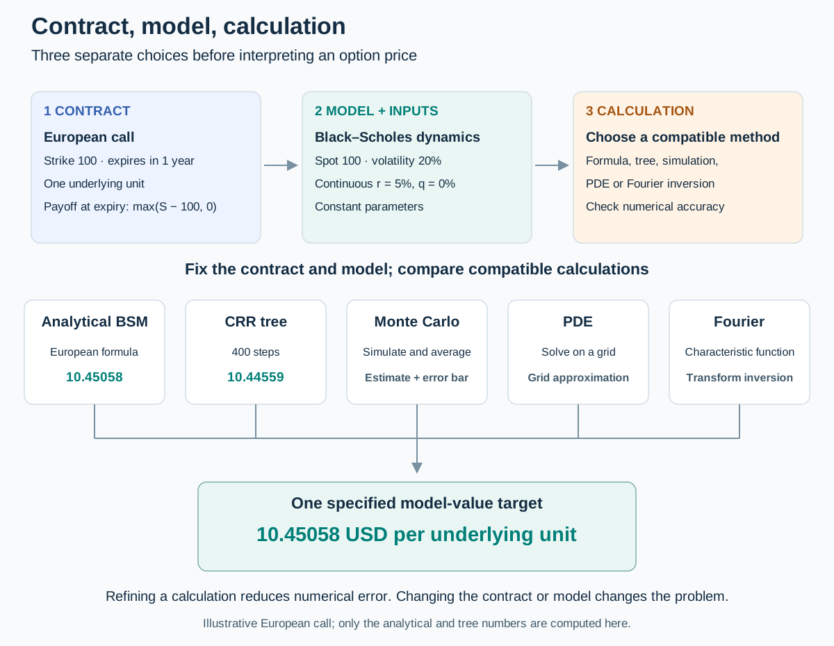
A diagram separates contract, model and calculation. One European call with fixed Black–Scholes dynamics can be valued analytically or approximated by a compatible tree, Monte Carlo, PDE or Fourier method. The analytical price is 10.45058 and the 400-step tree price is 10.44559.
Original illustration for the stated one-year call. The numerical labels show the analytical benchmark and the 400-step tree calculation. The other boxes identify compatible method families, rather than additional numerical results.
Owen's two numbers have the same target
His second implementation is a standard Cox–Ross–Rubinstein tree approximation. With N steps and Δt=T/N, it uses
u=eσΔt,d=u−1,p=u−de(r−q)Δt−d.
The parameters satisfy 0<p<1 for the benchmark grids. Each node rolls the two next values backward using
V=e−rΔt[pVup+(1−p)Vdown].
Start with the contractual terminal payoffs and apply that step until reaching today. No early-exercise comparison is inserted, because this is the European contract.
Calculation
Call value in USD per underlying unit
Analytical Black–Scholes benchmark
10.45058
CRR tree, 25 steps
10.52097
CRR tree, 100 steps
10.43061
CRR tree, 400 steps
10.44559
The 25-step result explains the original 10.52 quote. Increasing resolution brings the approximation closer to the continuous-time target. Tree errors can oscillate, including between odd and even step counts; refinement does not promise a smooth approach from one side.
These are not competing opinions about the correct model. They are calculations with different numerical resolution. The Black–Scholes model page develops the analytical benchmark, while the Monte Carlo page shows how a simulation estimate reports its sampling error. Agreement across independently checked methods is useful evidence about implementation accuracy.
It is not evidence that constant volatility describes the market perfectly.
When a different price is a different problem
Change European exercise to American exercise, and the contract changes. An American solver must compare continuation with immediate exercise where allowed. Feeding a European formula the same strike and expiry does not price that extra right. An American value is at least the corresponding European value under otherwise identical assumptions; the premium can be zero in particular cases.
Change Black–Scholes to Heston, and the dynamics change. Stochastic volatility introduces extra parameters and risk-neutral assumptions. A Fourier Heston calculation and a Black–Scholes formula are not two algorithms for one unchanged model. Even models calibrated to the same vanilla market quotes can disagree about an exotic payoff or its hedge: that is model risk.
Change the numerical settings, and the approximation changes. More paths reduce ordinary Monte Carlo sampling error but do not remove a wrong exercise rule or a monitoring-date error. A finer PDE grid does not repair an incorrect boundary condition. Prices may appear stable while their Greeks remain inaccurate.
When implementations disagree, first compare payoff, exercise, payment dates, units, rates, dividends and model parameters. Then inspect convergence and error estimates. Only after matching those specifications is the difference a meaningful numerical comparison.
Explore the benchmark with the right tool
SelfMadeQuant's Options Pricing tool is a free public European Black–Scholes tool. Use spot 100, strike 100, 365 days, volatility 20%, rate 5%, dividend yield 0%, and select call to reproduce the approximately 10.45 benchmark. Its heatmap varies spot and volatility. It does not currently implement the tree, Monte Carlo, PDE or Fourier alternatives discussed here.
If the contract vocabulary is new, start with the Options primer: the full lesson is free with a signed-in account. It distinguishes rights, payoff, profit and exercise style. For a structured route through replication, trees, finite differences and simulation, the Options Pricing Programme syllabus is public; full lessons require membership.
The numerical benchmark follows the European model and conventions documented in MathWorks' Black–Scholes reference. John C. Hull's Options, Futures, and Other Derivatives, Chapters 13, 15 and 21 in the edition held in the learning vault, grounds the tree limit, analytical model and numerical-method comparisons. The benchmark inputs, calculations and diagram here are original teaching material.