A percentile is a quantile with its probability level expressed out of 100. The 95th percentile is the threshold associated with probability . The level is a percentage; the threshold retains the variable's units. A 95th-percentile loss of USD 95 therefore contains two different pieces of information, even though both happen to use the number 95.
For a population with cumulative distribution function , use the lower generalised inverse convention:
The th percentile is . For a continuous, strictly increasing CDF, : exactly that share of probability lies at or below the threshold. With discrete outcomes, the CDF may jump past , so the equality need not hold. The 50th percentile gives a median; the inverse convention selects the lower endpoint if there is an interval of possible medians.
A loss limit is not the average bad day
Imagine a deliberately simple synthetic one-day loss model: has a uniform distribution between USD 0 and USD 100. Positive values mean losses, and equal-length intervals have equal probability. On that support, , with measured in USD. Therefore,
A desk using this model could call USD 95 its one-day 95% Value-at-Risk. It is a loss threshold under the assumed model, not a maximum loss or a promise about future trading days.
The overall mean loss is USD 50. Conditional on exceeding USD 95, the loss is uniform between USD 95 and USD 100, so its mean is
That upper-tail average equals 95% expected shortfall in this continuous model. The percentile only locates the boundary; it does not describe the severity of losses beyond it. For distributions with probability mass at the boundary, expected shortfall requires allocating the appropriate fraction of that mass rather than blindly conditioning on strict exceedance.
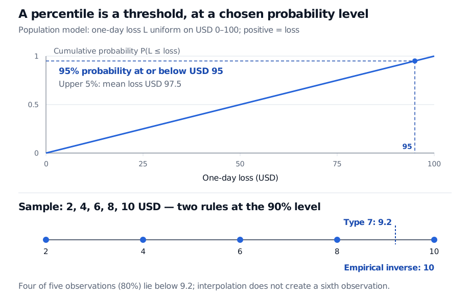
Original synthetic examples. The upper plot reads a population percentile from a CDF; the lower strip compares two sample estimation rules. Filled dots in the lower strip are observations.
Five observations do not define a unique interpolation rule
Now put the population model aside. Suppose the only data are five equally weighted observed losses, sorted into USD 2, 4, 6, 8 and 10. A sample quantile needs an explicit calculation convention.
Using R type 7 linear interpolation, set . At and , , so interpolate 60% of the way from the fourth observation to the fifth:
By contrast, the empirical inverse-CDF rule takes the first observed value whose cumulative sample proportion reaches 90%. At USD 8, that proportion is ; at USD 10, it is 100%. This rule therefore gives USD 10. R documents both rules, among nine supported algorithms.
Neither method makes exactly 90% of these observations fall below its answer. Four of five observations lie strictly below USD 9.2, and four lie strictly below USD 10. At or below USD 10, all five are included. An interpolated sample estimate need not itself be an observation or invert the empirical CDF exactly. NIST's discussion explains why the chosen estimation rule belongs with the reported percentile.
Read the boundary, units and horizon together
Ties make the “percentage below” shortcut especially unreliable. If a loss distribution assigns 96% probability to USD 0 and 4% to USD 100, its lower-inverse 95th percentile is USD 0. Zero probability lies strictly below it, 96% lies at or below it, and 4% lies above it. The percentile is well defined even though none of those shares equals 95%.
A percentile rank asks the reverse question: given a value, what share lies below it? That share needs its own convention for including ties. It is not the same object as the percentile threshold.
For a risk report, specify whether the variable is a loss or a return: high loss percentiles identify bad outcomes, while downside return risk sits at low return percentiles. Include the horizon, currency or return units, probability weights and sample method. A short historical sample also leaves substantial estimation uncertainty; changing the interpolation method cannot supply missing tail observations or establish that tomorrow follows the same distribution. The Empirical CDF and QQ-plots lesson develops sample proportions and distribution diagnostics; its full text requires membership, with a public preview available.
Sources
- Larry Wasserman, All of Statistics: A Concise Course in Statistical Inference (Springer, 2004), Example 7.14 — generalised inverse and empirical sample quantiles.
- R Core Team, Sample Quantiles, stats documentation — empirical inverse (type 1), linear interpolation (type 7) and the nine algorithm choices.
- NIST/SEMATECH, e-Handbook of Statistical Methods, §7.2.6.2: Percentiles — ordered observations and alternative percentile estimators.