A lognormal variable is the exponential of a normal variable. Translate log-return assumptions into positive prices, distinguish the mean from the median, and calculate model-based loss probabilities.
Lognormal distribution
A lognormal distribution describes a strictly positive random variable whose natural logarithm has a normal distribution. It arises when normally distributed log returns are converted into prices. A symmetric distribution of log returns becomes a price distribution with a longer right tail: prices have a floor at zero and no upper bound.
That transformation changes what “average” means. Exponentiating the average log return gives the median terminal price, not its expected value. This distinction matters when checking a price simulator, interpreting a forecast, or calculating the probability of losing money.
State the parameters on the right scale
Write
Y=lnX∼N(m,s2),X=eY,s>0.
Then X is lognormal. Here m is the mean of the logarithm and s is its standard deviation. Neither is the mean or standard deviation of X. Software packages use different lognormal parameter conventions, so check whether an input means a log mean, a scale or a level mean. NIST, for example, also describes a scale parameter equal to the median. We use m exclusively for the log mean below.
For a financial price it is cleaner to take the log of a dimensionless ratio:
L=ln(S0ST)∼N(m,s2),ST=S0eL.
The positive initial price S0 supplies the currency units. The parameters m and s refer to the whole stated horizon. They are not automatically annual quantities.
Because the exponential function increases, a price threshold K>0 becomes a normal threshold:
P(ST≤K)=Φ(sln(K/S0)−m),
where Φ is the standard normal cumulative distribution function. For K≤0, this probability is zero. No log of a nonpositive threshold is needed.
The corresponding density is
fST(x)=xs2π1exp[−2s2(ln(x/S0)−m)2],x>0.
The factor 1/x adjusts for the change of scale: equal intervals of log return map into wider price intervals at higher prices. Simply relabelling the horizontal axis of a bell curve would give the wrong price density.
A USD 100 position with three different averages
Suppose a hypothetical non-dividend-paying share starts at USD 100, and the assumed one-year physical distribution is
ln(ST/100)∼N(0.06,0.202).
This is a stipulated model, not a market estimate. Its mean log return is 0.06 and its log-return standard deviation is 0.20. The key level statistics are
Probability-weighted arithmetic average across outcomes
Terminal price variance
478.92 USD²
Spread on the price scale
The median follows directly from symmetry: half the log returns fall below m, so half the prices fall below 100em. For the mean, integrating eL against its normal density, or completing the square in the exponent, gives EeL]=em+s2/2. The extra factor es2/2 captures the effect of the right tail on the arithmetic mean. This is an instance of [Jensen’s inequality.
The model’s expected simple return is therefore e0.08−1=8.33%. The median simple return is e0.06−1=6.18%. Neither is exactly the 6% mean log return. Calling all three “the annual average return” would conceal materially different quantities.
A positive expected return also does not mean a loss is unlikely enough to ignore:
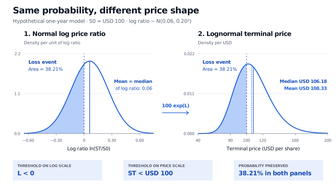
P(ST<100)=Φ(0.200−0.06)=Φ(−0.30)≈38.21%.
A normal log return becomes a skewed price distribution; the loss probability remains 38.21%, with median USD 106.18 and mean USD 108.33.
Original hypothetical one-year distribution, not market data. The increasing exponential transformation preserves the shaded event’s probability while changing the density shape and its units. Finite plotted ranges do not truncate either model.
Quantiles transform just as directly. For 0<p<1, the price quantile is
qp=S0exp(m+sΦ−1(p)).
The example’s 5th and 95th percentiles are USD 76.42 and USD 147.55. This central 90% model interval is asymmetric around both the median and the mean. It is a range for a future price under the assumed distribution, not a confidence interval for an estimated parameter.
How this connects to GBM
Geometric Brownian motion adds a model for the entire path. With constant physical price drift μ and volatility σ,
dSt=μStdt+σStdWt⟹m=(μ−2σ2)T,s2=σ2T.
For T=1 year and σ=0.20 per square root year, our m=0.06 implies μ=0.08 per year. The 8% instantaneous proportional price drift produces a one-year expected simple return of 8.33% through compounding. It is not the 6% expected log return. The half-variance correction follows from Itô’s lemma.
A lognormal distribution at one date does not, by itself, establish GBM dynamics, independent increments or a law for prices at other dates. Under the usual risk-neutral GBM used for European option valuation, the price drift is instead r−q, with continuous risk-free rate r and dividend yield q. That pricing distribution should not be presented as an investor’s physical forecast. The Black–Scholes model uses this distinction.
Useful structure, restrictive assumptions
Lognormality keeps prices positive, but it does not prevent severe losses: prices can approach zero. It also rules out an exact zero-price outcome, which can matter when modelling default or delisting. A shifted simple return R=ST/S0−1 has support above −100%; it is not itself a standard positive lognormal variable, and it is not normal either.
The model is a tractable baseline for multiplicative growth. Its suitability still depends on the variable and horizon. Jumps, changing volatility and departures from normal log returns can make its tail probabilities misleading. A portfolio sum of lognormal asset values is also generally not lognormal. Do not transfer the one-asset formulas to an arbitrary portfolio without another argument.
1. A hypothetical asset starts at USD 80. Over the next six months its log price ratio is normal with mean 0.03 and standard deviation 0.30. Find the median price, mean price and probability of ending below USD 80. The parameters already describe six months; do not annualise them.
Answer. The median is 80e0.03=82.44 USD, whereas the mean is 80e0.03+0.302/2=86.23 USD. The loss probability is Φ(−0.03/0.30)=Φ(−0.10)≈46.02%. Exponentiating 0.03 alone gives the median growth factor, so it misses the mean’s half-variance adjustment.
2. Another hypothetical asset starts at USD 120. Its one-year log price ratio has mean −0.02 and standard deviation 0.40. Must its expected simple return be negative?
Answer. No. Its median price is 120e−0.02=117.62 USD, below the starting price, but its mean price is 120e−0.02+0.402/2=127.42 USD. The expected simple return is e0.06−1=6.18%. A negative mean log return can coexist with a positive arithmetic expected return because the exponential transformation gives more weight to large positive outcomes.
Sources
John C. Hull, Options, Futures, and Other Derivatives, 9th Global Edition, §§15.1–15.3, pp. 344–347: lognormal stock prices, continuously compounded returns, and arithmetic versus log-return expectations.
NIST/SEMATECH e-Handbook: Lognormal Distribution: definition, density, parameter conventions and distribution functions. This article uses the unshifted distribution and states its own log-parameter notation.