The Sharpe ratio measures mean excess return per unit of return variability. Calculate it, distinguish population and sample ratios, and see when annualisation fails.
Sharpe ratio
The Sharpe ratio is mean excess return divided by the standard deviation of that excess return. It asks how much return an investment earns above a chosen financing benchmark for each unit of variability. A larger return alone does not imply a better Sharpe ratio: taking substantially more risk can raise the return while lowering the ratio.
For a stated holding period, let R be the investment's simple total return, including distributions, and Rf the cash return for the same period. Define the excess return X=R−Rf. The population ratio is
S=Var(X)E[X]=σXμX,σX>0.
Here, expected return describes a probability distribution, rather than one realised year's profit. Standard deviation measures fluctuations on both sides of the mean. The ratio therefore treats unusually large gains as variability too; it is not a measure of downside loss alone.
The usual benchmark is a risk-free rate or suitable cash proxy. Sharpe's broader formulation allows a return differential against another benchmark; against a risky investment benchmark, the corresponding mean-active-return-to-tracking-error measure is commonly called an information ratio. State the benchmark, rather than treating these names as interchangeable. Sharpe's original discussion explains this return-differential basis.
The fund with the bigger return loses the comparison
Imagine two funds and a certain annual cash return of 3%. The following are stipulated population moments of one-year returns, not estimates from a short performance record.
Annual quantity
Fund A
Fund B
Expected total return
11%
13%
Expected excess return
8%
10%
Standard deviation of excess return
16%
24%
Sharpe ratio
0.500
0.417
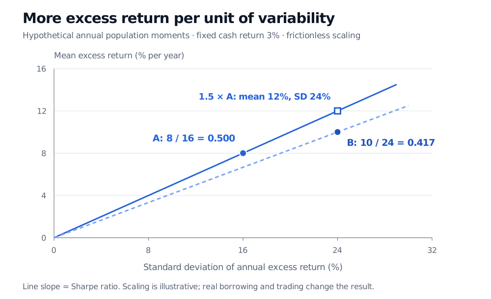
Fund A's ratio is 0.08/0.16=0.5: it offers half a unit of expected excess return for each unit of annual return variability. Fund B earns more above cash but requires proportionally more variability, so its ratio is 0.10/0.24≈0.417.
One exact construction for A is two equally likely annual excess returns, −8% and 24%. Their mean is 8%, and each is 16 percentage points from the mean. This is a two-state probability model, not a sample of two years; the population standard deviation is 16%.
Fund A has annual mean excess return 8%, standard deviation 16% and Sharpe 0.500. Fund B has 10%, 24% and Sharpe 0.417. Scaling A by 1.5 gives 12% mean excess return at 24% standard deviation.
Original hypothetical annual population moments. Cash earns a certain 3%. Lines show proportional scaling without costs or a borrowing spread.
The slope interpretation gives the comparison economic meaning. Invest 150% in A and borrow 50% at the same cash rate: the excess return becomes 1.5XA, so its mean is 12% and its standard deviation is 24%. At B's variability, the idealised A allocation has a higher expected excess return. Its Sharpe remains 0.5. Actual leverage introduces funding spreads, margin constraints and trading costs, so this proportional comparison requires those assumptions.
This does not make A the best addition to every existing portfolio. A fund's correlation with the investor's other holdings can matter more than its standalone ratio. The portfolio context is developed in Risk-Adjusted Performance Measures (full lesson requires membership; a public preview is available).
What a historical calculation actually estimates
A performance record gives observations xt=Rt−Rf,t, not the population mean and variance. For n≥2 equal-length periods, a common sample convention is
The n−1 convention belongs to the sample variance; using it does not make the estimated ratio unbiased. A short or favourable sample can produce a large estimate of a modest underlying Sharpe.
Match the inputs before calculating. Daily fund returns need daily cash returns in the same currency and on aligned dates. An annual quoted cash yield needs conversion using its stated compounding and day-count convention. If cash varies across observations, compute the standard deviation of Rt−Rf,t itself. Subtracting a constant leaves standard deviation unchanged; subtracting a variable cash series generally does not.
Use arithmetic mean excess returns in the numerator. Substituting compound annual growth rate creates a different statistic. For instance, consecutive returns of +20% and −20% have arithmetic mean zero but turn wealth of 100 into 96. Growth describes the compounded path; the Sharpe numerator averages period return differentials.
Costs belong in the return series being assessed. If a certain annual cost of 2 percentage points is deducted from A's model return, its mean excess return falls from 8% to 6%, with unchanged variability in this deliberately fixed-cost case. Sharpe falls to 0.06/0.16=0.375. Actual transaction costs vary with trading, so they can alter both numerator and denominator. Do not deduct them again from returns already reported net of those costs.
The annualisation trap
Suppose daily excess returns have mean 0.04% and standard deviation 1%. Their daily ratio is 0.04. The familiar annualised calculation is
2520.010.0004≈0.635.
Why the square root? For a sum of q excess returns with a constant mean and variance, and zero covariance across different dates, the mean is qμX and the standard deviation is qσX. Independence with identical distributions is sufficient, but zero serial covariances and stable moments already give this moment identity.
For a covariance-stationary series, let γk=Cov(Xt,Xt−k). Then
Var(t=1∑qXt)=qσX2+2k=1∑q−1(q−k)γk.
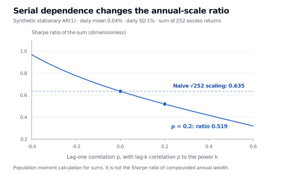
Positive serial covariances increase the denominator relative to the zero-covariance calculation. For a synthetic stationary AR(1) model with γk=σX2(0.2)k, keeping the same daily mean and standard deviation gives a 252-day sum-based ratio of approximately 0.519, rather than 0.635.
For synthetic daily excess returns with fixed mean 0.04% and standard deviation 1%, the 252-period sum-based Sharpe is 0.635 with zero serial correlation and 0.519 at lag-one correlation 0.2.
Original population calculation for a stationary AR(1) model. Lag-k correlation is rho to the power k. The dashed line uses zero-autocovariance square-root scaling at every rho; the solid curve includes the model's covariances.
Summing daily simple excess returns is not compounding annual investment and cash wealth. The square-root formula is a conventional scaling under stated assumptions, not a general identity for the Sharpe ratio of compounded annual returns. Lo's original paper, especially “Time Aggregation,” makes both the serial-correlation issue and the ignored-compounding assumption explicit.
Reading a reported number without overreading it
A negative ratio means mean return fell below the benchmark when variability is positive. It does not mean variability is negative. Negative ratios also make naive rankings awkward: raising volatility while holding a negative mean fixed pushes the ratio toward zero, although the investment has become more variable. If standard deviation is zero, the ordinary ratio is undefined, including the zero-over-zero case. A flat or stale-marked record is not evidence of infinitely good performance.
Normality is not required to define a finite-moment Sharpe ratio. It matters for particular statistical tests and for whether mean and variance adequately describe what investors care about. A strategy selling crash protection can show smooth gains until a rare loss arrives. The same Sharpe can conceal very different tail exposures, liquidity and maximum drawdown. The Sortino ratio changes the variability measure to shortfall relative to a target; it does not remove estimation uncertainty.
Finally, the highest Sharpe among many backtests can owe much of its ranking to good luck. Report the observation frequency, dates, benchmark, cost basis, annualisation method and research-selection process alongside the ratio. Compare like with like, and inspect the return path that produced the summary.
Sources
William F. Sharpe (1994), “The Sharpe Ratio”, Journal of Portfolio Management, Fall, pp. 49–58. Author-hosted reprint; ex ante versus ex post, differential returns and portfolio context.
Andrew W. Lo (2002), “The Statistics of Sharpe Ratios”, Financial Analysts Journal 58(4), pp. 36–52. Original paper; estimation and time aggregation, especially pp. 40–42.
Elton, Gruber, Brown and Goetzmann, Modern Portfolio Theory and Investment Analysis, 9th ed. (2014), Chapter 26, pp. 665–667 and 669–670. Sharpe measure, portfolio context and asymmetric-return limitations.