The Sortino ratio measures average return above a chosen target per unit of downside deviation from that target. It is useful when falling short of an investment objective matters differently from exceeding it: a large gain raises the numerator but contributes no shortfall to the denominator.
The target is often called the minimum acceptable return, or MAR. It need not be zero or a risk-free rate. A strategy returning a positive amount can still fall short of a positive target. The choice of target is part of the investment question, not an innocuous reporting setting.
Unlike the Sharpe ratio, which uses the standard deviation of matched excess returns, Sortino focuses on target shortfalls. Both are performance summaries. Neither proves that a strategy has a persistent edge.
Start with the convention
For equally spaced simple returns and a fixed target at the same frequency, define
Then the historical, periodic Sortino ratio is
This article uses the all-observation lower-partial-moment convention: divide by all periods, even those with zero shortfall. Do not centre returns at their sample mean, calculate the standard deviation of the negative returns, or apply an adjustment. These operations answer different questions. Rollinger and Hoffman's author paper, hosted by CME, explicitly specifies the all-period root-mean-square calculation.
The corresponding population quantity replaces the empirical averages with expectations: . Its square is the second lower partial moment about . A historical calculation estimates this object; six observations do not reveal the full future distribution.
A small gain with an uncomfortable bad month
An analyst reviews six hypothetical monthly simple returns, net of the strategy's stated fees and trading costs. The investment committee sets a monthly MAR of 0% before examining the record.
| Month | Return | Shortfall below 0% | Squared shortfall, decimal-return units |
|---|---|---|---|
| 1 | +2% | 0 | 0 |
| 2 | −1% | 1% | 0.0001 |
| 3 | +3% | 0 | 0 |
| 4 | −4% | 4% | 0.0016 |
| 5 | +1% | 0 | 0 |
| 6 | 0% | 0 | 0 |
Here “shortfall” is the positive magnitude ; squaring it gives the same denominator as the signed negative part in the formula.
The arithmetic sample mean is
or 0.16667% per month. It is not the compounded six-month return or a compound growth rate. Downside deviation is
or 1.68325% per month. The monthly Sortino is therefore
The numerator measures average return above the target across all months. It is not the mean gain of winning months. The denominator gives the −4% month sixteen times the squared-shortfall contribution of the −1% month.
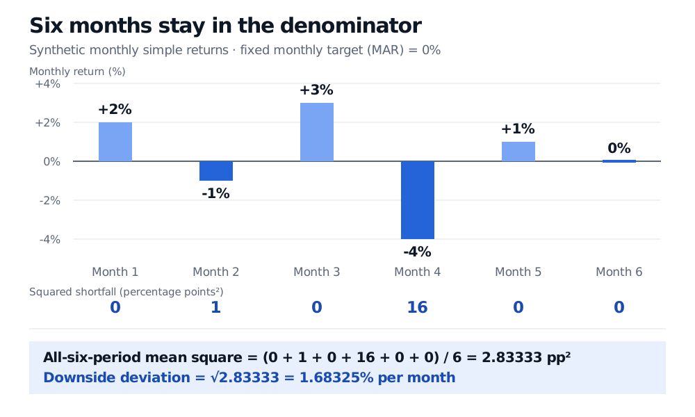
Original synthetic monthly simple-return example. Monthly MAR is zero; all six observations remain in the downside-deviation divisor.
Why dividing by two changes the statistic
There are two below-target months. Dividing their squared shortfalls by two gives a conditional shortfall RMS of , and a ratio of 0.05717. This is a different convention, not an alternative computation of 0.09901. It is also distinct from centring the two losses at their own average and taking their standard deviation.
When observations breach the target,
The all-period measure combines the observed frequency of shortfalls with their conditional squared size. Dropping the zero shortfalls removes the frequency component. Always inspect a provider's formula before comparing reported ratios.
The target is an economic choice
Suppose the committee instead requires 1% per month, using the same six returns. Month 6, with a zero return, now has a 1 percentage point shortfall. The two losing months miss the target by 2 and 5 percentage points. Month 5 exactly meets the target and contributes zero.
The downside deviation rises to 2.23607% per month, while average return above target becomes −0.83333% per month. Their ratio is −0.37268. The strategy did not change; the question did.
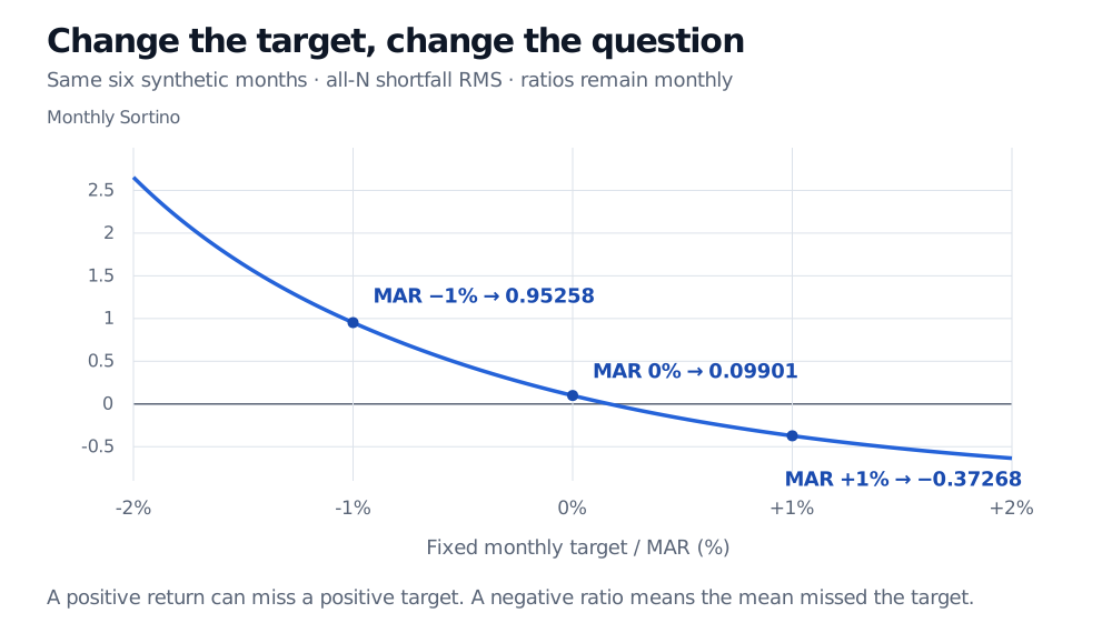
Original calculation using the same six synthetic observations and the all-N lower partial moment. Target choice changes both numerator and shortfalls.
A negative ratio means the sample mean missed the target. It is not a shortfall probability: 0.09901 does not mean a 9.901% chance of success. Nor is there a universal “good Sortino” cutoff independent of target, period, strategy and sample length. With a negative numerator, increasing the denominator can move a ratio closer to zero; do not interpret every numerical improvement as a better investment.
Preserve the horizon, then investigate the record
Match returns and target by frequency, currency, nominal or real basis, and fee treatment. An annual effective target can be translated to an equivalent compounded monthly rate using . That translation does not make a sequence of monthly target tests equivalent to testing an annual objective. Gains and losses can offset inside the year.
Do not mechanically multiply monthly Sortino by and call it an annual Sortino. The downside operator is nonlinear: the shortfall of an aggregated return is not the sum of its period shortfalls. Even independence alone does not supply the required lower-partial-moment scaling rule. For an annual-horizon measure, specify how annual returns and the annual target are formed and estimate downside risk at that horizon, acknowledging the smaller sample. Kidd's CFA Institute article discusses the material effect of calculation and horizon choices.
The six-month example deliberately has little evidence behind it. A strategy selling crash insurance may produce many small gains before its large loss arrives. An observed downside deviation of zero makes the ratio undefined under the formula here; software may display infinity, but that is not evidence of no risk. Stale or smoothed valuations can also hide adverse movements.
Sortino treats different orderings of the same returns identically. Maximum drawdown, funding needs and time underwater depend on sequence. Inspect these alongside leverage, liquidity and plausible unobserved losses. Stress scenarios add information that a favourable historical ratio cannot provide.
Finally, retain the search history. Selecting the best Sortino from many backtests, then advertising its in-sample value, invites overfitting. Choose the target for economic reasons, evaluate on untouched data and report sensitivity to window and costs. The membership lesson Backtest Evaluation develops the broader evidence package: net returns, drawdowns, concentration, uncertainty and research history. Its public page provides a preview.
Sources
- Elton, Gruber, Brown and Goetzmann, Modern Portfolio Theory and Investment Analysis, 9th edition (2014), Chapter 4, p. 46 — semivariance and lower partial moments. This article uses a fixed target rather than centring downside risk on the sample mean.
- Thomas N. Rollinger and Scott T. Hoffman, Sortino: A ‘Sharper’ Ratio, pp. 3–5 — author paper defining target downside deviation, retaining all observations and distinguishing it from standard deviation of losses.
- Deborah Kidd, CFA, The Sortino Ratio: Is Downside Risk the Only Risk that Matters? (2012), pp. 2–3 — target, implementation differences, horizon sensitivity and limits of historical downside estimates. Numerical examples and figures here are original.