Read a residual as observed minus fitted, calculate signed fund-return misses, and distinguish OLS training identities from assumptions about errors and forecasts.
Residual
A residual is an observed value minus the value assigned to it by a fitted model:
ei=yi−y^i.
A positive residual means the observation lies above the fitted value; a negative one means it lies below. In a fund-return regression, it is the part of the observed return left over after subtracting the fitted factor contribution and the fitted intercept. It is not automatically investment skill, a pricing error or a tradeable signal.
The fund did worse than its model on a flat market
Consider five synthetic weeks of market and fund excess returns, each measured relative to the same risk-free benchmark. Fit a linear regression of fund return on market return using ordinary least squares, including an intercept. The return entries below are percentages: an entry of 2 means a 2% return. Their differences are percentage points, abbreviated pp.
The fitted relationship is
y^i=1+1.2xi.
The intercept is 1 pp per week; the slope is dimensionless because both returns use the same units. This is a contemporaneous exposure fit, not a forecast that could have been made before seeing that week's market return.
Week
Market return (%)
Fund return (%)
Fitted fund return (%)
Residual (pp)
A
−2
−1
−1.4
+0.4
B
−1
0
−0.2
+0.2
C
0
0
1.0
−1.0
D
1
2
2.2
−0.2
E
2
4
3.4
+0.6
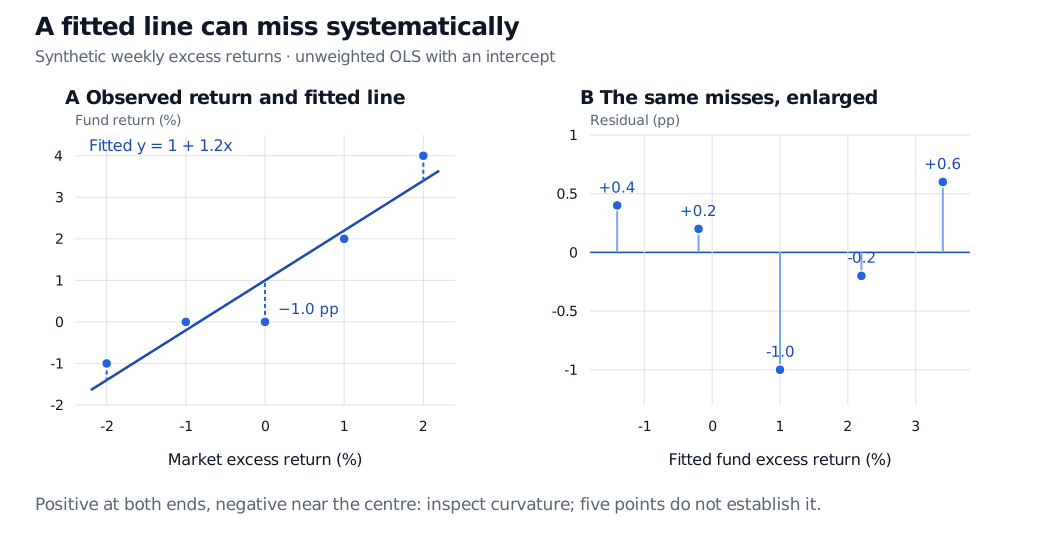
In week C the market and fund excess returns were both zero. Yet the residual is −1 pp, because the fitted intercept assigned the fund a 1% excess return even at a flat market. Subtracting only the slope contribution would incorrectly report zero. Conversely, week A has a positive residual despite a negative fund return: the fund lost less than the fitted relationship implied.
Synthetic five-week excess-return fit y = 1 + 1.2x and residual plot. Signed residuals are +0.4, +0.2, −1.0, −0.2 and +0.6 percentage points; the largest absolute miss is at the flat-market observation.
Original synthetic data. Left: the vertical differences from the fitted line. Right: the same residuals against fitted returns on an enlarged scale; both panels use the same five observations.
The residual plot removes the fitted upward trend so the remaining shape is easier to see. Here the two ends are positive and the middle is negative: a reason to investigate curvature in the conditional relationship, not proof of it from five observations. A widening residual band in a larger sample would raise a different question—whether error variance changes with the level of the predictor. A plot in time order is needed to investigate runs or volatility clustering; the horizontal axis above is fitted return, not time.
For a first hand calculation, Basic Statistics and Regression builds the fitted line from covariance and variance. The public page is a preview; the full lesson is free with a signed-in account.
Squaring prevents positive and negative misses from cancelling. Nevertheless, cancellation in the unsquared residuals is an unavoidable fitting identity. The first-order conditions for an unweighted OLS fit with an intercept and one nonconstant predictor give
i∑ei=0,i∑xiei=0.
The example satisfies both exactly. In matrix form, the corresponding statement is X⊤e=0: the residual vector is orthogonal to every included design column. These are properties of the training sample and fitting method. The zero-sum property need not hold when the intercept is omitted; weighted least squares instead supplies weighted normal equations.
Orthogonality removes the sample linear association with included regressors. It does not establish independent, normally distributed or constant-variance disturbances, nor rule out a nonlinear pattern such as the one suggested above. Even with a fixed design and independent errors of common variance, fitted residuals share estimated coefficients and generally depend on one another. Under that model their covariance matrix is σ2(I−H), where H is the OLS projection matrix. A small raw residual at a high-leverage observation can partly reflect the fitted line being pulled towards that observation.
The Linear Regression lesson derives the normal equations and connects residual geometry to coefficient uncertainty. Its public preview is open; the full lesson requires membership.
Three different deviations
A population error refers to an underlying relationship, for example εi=yi−(α+βxi) when the population conditional mean is linear. The true coefficients are generally unknown. The training residual instead uses estimated coefficients, ei=yi−(α^+β^xi), so it is observable after fitting and is only a proxy for that error.
A forecast error compares a later realised outcome with a forecast fixed using information available at the forecast origin. It reflects both new disturbances and uncertainty or misspecification in the forecast. It need not average to zero on held-out data, and its predictor inputs must actually have been available when the forecast was issued. Re-fitting on the evaluation sample would erase this distinction.
For finance, the question is therefore not just whether residuals are small. It is whether their structure exposes an omitted exposure, changing risk or a weak model—and whether any apparent opportunity survives a genuinely separate evaluation with realistic timing and costs.
Sources
Chris Brooks, Introductory Econometrics for Finance, 2nd edition, Cambridge University Press, 2008, §2.3, pp. 31–33 (least squares and signed residuals), and §2.4.2, pp. 37–38 (population and sample regression functions).