The intercept is the fitted response at a chosen zero. See why a 1% return intercept differs from an observed return, changes under recentering, and is not automatically alpha.
Intercept
The intercept is a model's response value when its explanatory variables are zero. For a straight line y=a+bx, it is a: the height where the line crosses the vertical axis. In a fitted linear regression, a^ is the fitted response at that chosen origin, not necessarily an observed outcome.
That distinction matters on a fund report. A positive intercept can describe what a fitted return relationship assigns to a flat market. It does not establish a fixed profit the fund earns independently of market conditions.
A flat market does not force the fund onto the line
Suppose five synthetic months produce these market and fund simple raw returns, displayed in percent. Thus the entry 2 means a return of 2%, or 0.02 in decimal units.
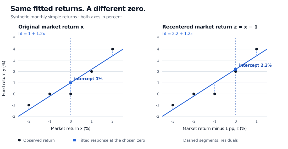
The intercept is a 1% fitted monthly fund return at a 0% market return. But month C actually returned zero: its residual, observed minus fitted, is 0−1=−1 percentage point. At a 2% market return, the fitted fund return is 1+1.2(2)=3.4%; the actual 4% return leaves a 0.6-percentage-point residual. The intercept belongs to the line; individual observations can sit above or below it.
The calculation comes from the sample means and centered sums:
The sums have squared-percentage-point units; their ratio is dimensionless because both returns use the same scale. The intercept has the response's units. In decimal returns the very same fit is y^=0.01+1.2x, so reading the coefficient without its units would change its apparent size a hundredfold.
For a gentler introduction to these calculations, Basic Statistics and Regression covers fitted lines and residuals; the full lesson is free with a signed-in account.
Move zero, move the intercept
Now describe the market relative to a 1% month. With returns still entered as percent numbers, define z=x−1. Substituting x=z+1 gives
y^=1+1.2(z+1)=2.2+1.2z.
The new intercept is 2.2%, because z=0 now means an original market return of 1%. Every fitted fund return and every residual stays the same. The slope stays 1.2. Merely changing the reference point has not improved the fund's performance.
Synthetic monthly raw returns fitted by a line of slope 1.2. With original market returns the intercept is 1%; after subtracting 1 percentage point from every market return the intercept is 2.2%. Black observations and fitted returns retain the same heights.
Original synthetic example. Blue squares mark fitted responses at each chosen zero; black circles are observations. Recentring changes the intercept while preserving fitted values.
More generally, replacing x by z=x−c changes an intercept from a to a+bc. Centering at the sample mean makes the fitted intercept equal yˉ. In multiple regression the intercept is the fitted response when all included predictors equal zero, so the reference point can be a combination scarcely represented in the sample. If zero lies far outside the observed range, the intercept is an extrapolation even when the line fits the available observations well.
When can it be called alpha?
In a specified asset-pricing regression of the fund's excess return on market excess return, the intercept is commonly called alpha. Our table instead uses raw returns. If the risk-free return is the same constant rf each month, then changing both variables to excess returns yields an intercept
α^=a^+(b^−1)rf,
with all returns expressed in the same units. If rf varies, subtract it observation by observation and refit; the simple constant-shift identity no longer applies. Subtracting a benchmark from a predictor alone, as in the recentering example, is also different from subtracting the risk-free return from both series.
Even a correctly defined alpha estimate is conditional on the chosen factors, period, sample and return conventions. Omitted exposures, fees, selection and estimation error can affect it. A monthly intercept is not automatically an annual compounded performance measure. Nor does an intercept identify a causal effect or guarantee a tradable return.
Including a freely estimated intercept makes unweighted OLS residuals sum to zero in sample. Forcing the intercept to zero imposes a different model and generally changes the slope and predictions; it requires an economic or modelling justification. Linear Regression develops the normal equations, inference and diagnostics (public preview; full lesson requires membership).
Sources
James, G., Witten, D., Hastie, T. and Tibshirani, R. (2021). An Introduction to Statistical Learning: with Applications in R, 2nd ed., §§3.1–3.1.2: fitted coefficients, least squares and coefficient uncertainty.