The residual sum of squares (RSS) adds the squared differences between observed outcomes and their fitted values. It measures how much a model misses the observations, in squared response units:
A residual is an observed fitting discrepancy; the model's unobserved population error is a different object. RSS is nonnegative and equals zero exactly when every fitted value matches its observation. Squaring prevents positive and negative misses from cancelling and gives larger misses disproportionate weight.
Ordinary least squares chooses coefficients to minimise this sum within a specified linear model. Computing that fit requires no normality assumption. Whether the chosen model gives useful forecasts or valid uncertainty statements requires further evidence.
Five weeks of unexplained fund returns
Suppose a risk analyst fits a fund's weekly excess returns to the same weeks' market excess returns. These are synthetic observations, quoted in percent: an entry of 2 means a 2% return. Residual differences are measured in percentage points (pp).
The fitted intercept is 1 pp and the slope is 1.2, giving the numerical fitted-return equation when returns are entered in percent.
| Week | Market (%) | Fund (%) | Fitted (%) | Residual (pp) | (pp²) |
|---|---|---|---|---|---|
| 1 | −2 | −1 | −1.4 | +0.4 | 0.16 |
| 2 | −1 | 0 | −0.2 | +0.2 | 0.04 |
| 3 | 0 | 0 | 1.0 | −1.0 | 1.00 |
| 4 | 1 | 2 | 2.2 | −0.2 | 0.04 |
| 5 | 2 | 4 | 3.4 | +0.6 | 0.36 |
| Total | 0 | 1.60 |
The signed residuals sum to zero, but the fit is plainly imperfect. RSS is 1.60 pp², with week 3 contributing 1 pp², or 62.5% of the total. Its negative sign disappears upon squaring; the original residual ledger is still needed to see whether the model overestimated or underestimated a return.
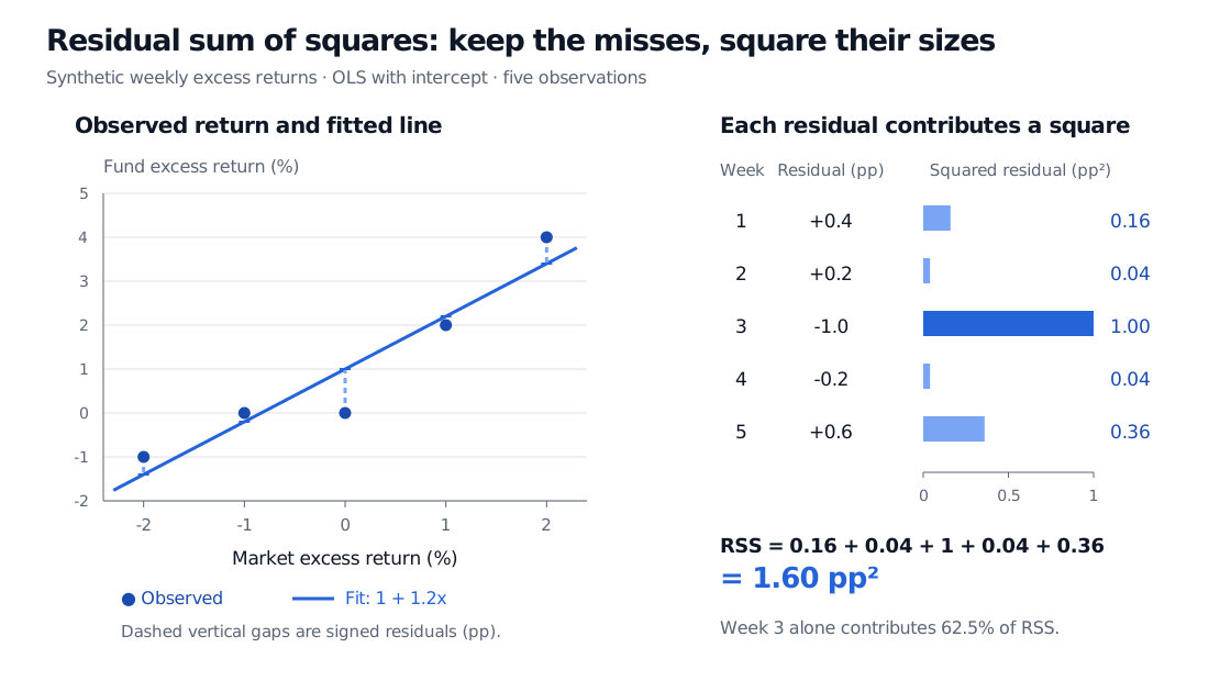
Original synthetic excess-return example. Vertical gaps show residuals; the separate bars show their squared contributions. All five observations are included in the fit.
This is a contemporaneous exposure fit: the same week's market return need not be known when a fund-return forecast must be made. A small RSS here would not establish a tradable signal. For a fuller derivation and a factor example, read Linear Regression; the public page provides a preview, and the full lesson requires membership.
One numerator, different questions
RSS is a sum, not a variance or an average error. For this fit, observations and fitted coefficients, including the intercept:
| Quantity | Calculation | Meaning |
|---|---|---|
| Training mean squared error | pp² | Average squared discrepancy on the fitted observations |
| Training root mean squared error | pp | Training error scale in the response's original units |
| Residual variance estimate | pp² | Estimate of a common population noise variance, under the conditions below |
| Residual standard error | pp | Square root of that variance estimate |
The mean squared error label needs context: an ANOVA table often calls its error mean square or MSE, whereas a training-loss report commonly means . Read the denominator. Neither is obtained by dividing by simply because the residuals average zero: the fitting procedure has used two coefficient degrees of freedom here.
For a fixed, full-column-rank design matrix with columns, the unbiasedness claim needs a correctly specified conditional mean and spherical errors:
“Spherical” means equal finite error variances and zero error covariances between distinct observations, conditional on . With the OLS projection matrix, the residual vector is . Its expected squared length is
That is why dividing by estimates without bias. Normality is unnecessary for this expectation identity; it enters the usual exact Gaussian regression distribution theory. Also, taking the square root does not make an unbiased estimator of .
Heteroskedasticity, autocorrelation or a misspecified conditional mean can invalidate the simple noise-variance interpretation. RSS remains computable, but its size alone cannot validate those assumptions or supply a confidence interval. Regression Assumptions and Diagnostics connects these failures to residual checks and covariance estimates; a public preview is available and the full lesson requires membership.
Read the formula before the acronym
RSS is also commonly called SSE, the error sum of squares. SSR is ambiguous: some authors mean sum of squared residuals, while an ANOVA table may mean regression sum of squares, the explained component. Peijie Hou's University of South Carolina notes use SSE for residual variation and SSR for explained variation. Check the defining formula before translating software or textbook output.
For unweighted in-sample OLS with an intercept, orthogonality gives the centred decomposition
In the five-week example the three sums are pp². Thus the coefficient of determination is . The model accounts for 90% of this sample's centred return variation; that statement carries no causal, forecasting or significance guarantee. Without an intercept, or when evaluating frozen coefficients on held-out data, do not assume the same centred orthogonal decomposition.
When a lower RSS is informative
Compare RSS values on the same response, observations and units. If the returns above are entered as decimals instead of percent, residuals shrink by 100 and RSS shrinks by 10,000, to 0.00016 decimal-return squared. The fit has not improved. A longer sample also changes what is being summed, so its raw RSS is not directly comparable with a shorter sample's.
On a fixed dataset, enlarging an unweighted OLS model's regressor space can only decrease or leave unchanged its minimum RSS: the old fit is still available with the extra coefficients set to zero. This algebraic improvement can accompany overfitting. Evaluate genuine forecasts on later or otherwise appropriately held-out observations, using coefficients estimated without those outcomes and predictors available at the forecast origin.
Finally, RSS compresses an entire residual pattern into one number. Inspect the signed residuals, their time order and their relationship to fitted values. The same sum can hide curvature, bursts of volatility or one dominant miss. It is a useful fitting criterion and a component of statistical calculations, not a certificate that a model is sound.
Sources
- Gareth James, Daniela Witten, Trevor Hastie and Robert Tibshirani, An Introduction to Statistical Learning with Applications in R, 2nd ed. (2021), §§3.1.1 and 3.1.3, equations 3.3 and 3.15–3.17: RSS, residual standard error and .
- John A. Rice, Mathematical Statistics and Data Analysis, 3rd ed., §§14.3 and 14.4.3, Theorem A: matrix least squares and the unbiased residual variance estimate under uncorrelated constant-variance errors.
- NIST/SEMATECH e-Handbook of Statistical Methods, §4.4.3.1, “Least Squares”: squared-residual minimisation and residual standard deviation with a coefficient-count denominator.
- Peijie Hou, University of South Carolina, STAT509: Simple Linear Regression, slides 11 and 19–21: SSE/SSR conventions, variance estimation and ANOVA decomposition.