R-squared compares a model’s squared error with a mean-only fit. Work through a fund-return regression, the OLS variance decomposition and a negative score on later observations.
Coefficient of determination
The coefficient of determination, usually written R2 and called R-squared, measures how much squared prediction error a fitted model removes relative to predicting the sample mean. For an in-sample ordinary least-squares regression with an intercept, it is also the fraction of the response's centred variation accounted for by the fitted values.
A risk analyst might regress a fund's weekly excess returns on the market's excess returns. A high R² says the fitted market exposure accounts for much of the fund's variation in those weeks. It does not say that the fund earns a high return, that the market causes its moves, or that tomorrow's return can be forecast before the market moves.
The comparison hidden in the denominator
For observed responses yi, fitted values y^i and sample mean yˉ, define
SSE=i=1∑n(yi−y^i)2,SST=i=1∑n(yi−yˉ)2.
Here SSE is the residual sum of squares, also called RSS; SST is the total centred sum of squares. Provided SST>0,
R2=1−SSTSSE.
SST is precisely the squared error incurred by predicting yˉ for every observation. Thus R² compares two errors on the same response and observations. It has no units: changing returns from percent to decimals changes both sums of squares by the same factor. It is not the percentage of observations predicted correctly or the probability of a profitable trade.
Under the usual centred in-sample OLS convention:
R2=1 means every fitted value equals its observed response.
R2=0 means the fitted model achieves the same squared error as the sample-mean fit.
If all responses are equal, SST is zero and this ratio is undefined. A software replacement of that result by zero or one is a reporting convention; scikit-learn's documentation makes its default replacement explicit.
Five weeks on a risk desk
Consider these synthetic, matched weekly excess returns. The market and fund returns refer to the same weeks and use the same risk-free-return subtraction. All entries below are percentages; residual differences are percentage points.
Week
Market x
Fund y
OLS fitted fund return
Residual y−y^
1
−2.0%
−1.0%
−1.2%
+0.2 pp
2
−1.0%
0.0%
−0.1%
+0.1 pp
3
0.0%
1.0%
1.0%
0.0 pp
4
1.0%
1.0%
2.1%
−1.1 pp
5
2.0%
4.0%
3.2%
+0.8 pp
The means are xˉ=0 and yˉ=1 in percent units. The OLS slope is 11/10=1.1 and the intercept is one percentage point, giving
y^=1+1.1x.
The slope describes the fitted market beta; R² describes fit. These answer different questions. The squared residuals sum to
SSE=0.22+0.12+02+(−1.1)2+0.82=1.9.
The fund's deviations from its mean are (−2,−1,0,0,3) percentage points, so
Both sums use percentage-points-squared units. The fitted line reduces squared error by 86.43% relative to the constant 1% fit on this sample; 13.57% remains as residual squared error. Those shares do not describe an expected future hedge performance. Five observations make the arithmetic inspectable, rather than establishing a stable relationship.
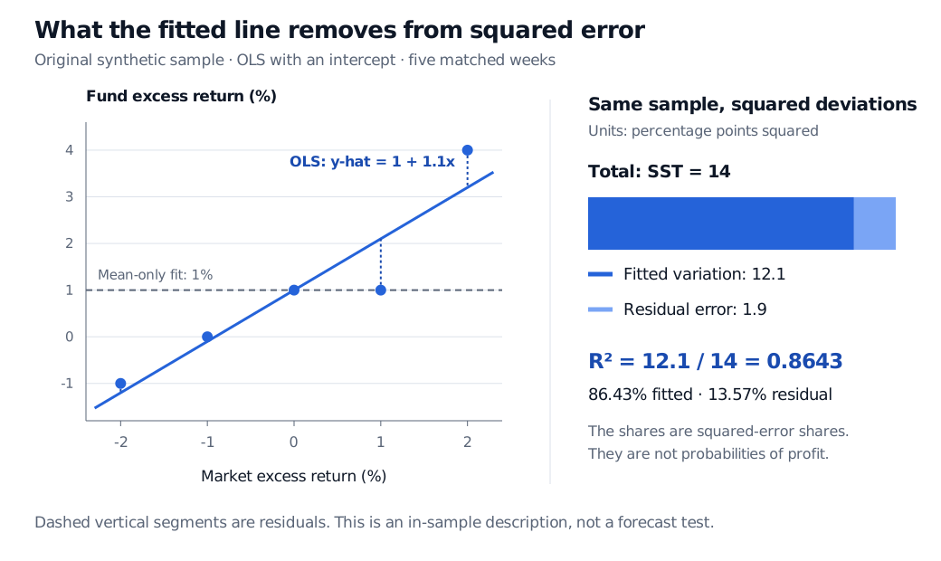
Five synthetic weekly market and fund excess-return pairs fitted by y-hat = 1 + 1.1x in percent units. A mean-only fund fit is 1 percent. Total squared deviation 14 equals fitted variation 12.1 plus residual error 1.9 in percentage points squared, giving R-squared 0.8643.
Original synthetic five-week sample. The line includes an intercept; vertical dashed segments are residuals. The bar decomposes squared deviations on these same observations.
Why “explained variation” needs conditions
Write each centred response as
yi−yˉ=(y^i−yˉ)+ei,ei=yi−y^i.
Squaring and summing would ordinarily leave a cross term. For unweighted in-sample OLS with an intercept, the normal equations make residuals orthogonal to every fitted regressor, including the constant. Consequently
This is why R2 equals fitted variation divided by total variation and lies between zero and one here. The identity is algebraic. It requires neither normally distributed errors nor homoskedasticity, independence or a correctly specified economic model. Those are separate matters for estimation and inference. Penn State's regression course develops the sum-of-squares interpretation and cautions about reading too much into the coefficient.
An omitted intercept, constrained or penalised coefficients, different fitting weights, or evaluation on new observations can break this particular orthogonality argument. Weighted regression needs matching weighted definitions. Some software reports an uncentred R² without an intercept, using ∑iyi2 as the denominator; that is a different baseline and should not be compared directly with centred R².
In simple linear regression with an intercept and nonconstant x and y, R² equals the square of their sample correlation. Squaring discards the slope's sign. This identity does not make an arbitrary prediction score the square of a correlation: biased or badly scaled predictions can correlate strongly with outcomes while having large squared errors.
A negative score on later observations
Freeze the five-week training coefficients. Suppose three later weeks have market returns of (−1,0,1) percent and fund returns of (0,0,1) percent. The frozen line predicts (−0.1,1,2.1) percent; do not refit it on these weeks.
Its test squared error is 0.12+(−1)2+(−1.1)2=2.22 percentage points squared. The test fund mean is 1/3 percent and its centred total sum of squares is 2/3. Therefore the test-mean version of the score is
Rtest2=1−2/32.22=−2.33.
The negative value says the frozen model has more squared error than the constant test-sample mean. It is not a negative explained-variance share, and it should not be clipped to zero. As the official scoring documentation notes, a prediction R² can be negative despite its name.
The denominator also deserves scrutiny. The test mean is available only after observing the test outcomes. For a genuine forecast comparison, specify a benchmark forecast bt using only information available at the forecast origin, and report
1−∑t(yt−bt)2∑t(yt−y^t)2,
when the denominator is positive. That benchmark-relative score need not equal the test-mean R². In this example, predicting the fixed training mean of 1% for each later week gives benchmark squared error 2, and the relative score becomes 1−2.22/2=−0.11. The benchmark changes the question, so name it alongside the score.
The return-on-return example is contemporaneous: the same week's market return is usually unknown when a weekly forecast must be issued. Using it can describe exposure after the week ends. Claiming a tradable forecast requires predictors available before the target period, suitable later evaluation, and protection against look-ahead bias.
Read R² alongside the question being asked
For a nested, unweighted OLS model fitted to the same observations with an intercept, adding regressors cannot increase the minimum SSE. Ordinary in-sample R² therefore cannot fall, even when the additional predictor contributes no dependable future information. Adjusted R-squared accounts for parameter count, but it still does not replace a genuine forecast test or prevent overfitting.
A useful report pairs R² with the response definition, observation window, intercept and weighting convention, error magnitude in meaningful units, and residual diagnostics. Compare models on the same target and sample: a log-price fit and a daily-return fit answer different questions. Shared trends in price levels can produce an impressive coefficient through spurious regression.
Finally, “explained” is a decomposition label, not a causal finding. Common drivers, reverse causation or selection can create a high fit. A low R² can still accompany an economically useful small forecast improvement; a high R² can coexist with no useful trading opportunity after timing and costs. There is no universal pass mark.
For the fitting mechanics, Basic Statistics and Regression is available in full with a free signed-in account. Linear Regression develops the projection and R² identities; Forecast Evaluation develops dated benchmark comparisons and loss functions. Both have public previews; their full lessons require membership.
Sources
Gareth James, Daniela Witten, Trevor Hastie and Robert Tibshirani, An Introduction to Statistical Learning: with Applications in R, 2nd edition (2021), §3.1.3, pp. 69–71, and §3.2.2, pp. 79–80 — residual versus total sums of squares, simple-regression correlation identity and training-fit behaviour as predictors are added.