Adjusted R-squared penalises in-sample regression fit for estimated parameters. Calculate it, see a zero-coefficient factor lower the score, and distinguish fit from forecasting.
Adjusted R-squared
Adjusted R-squared measures the fit of a linear regression after allowing for the number of parameters estimated from the sample. It replaces the raw error and total sums of squares in R-squared with quantities divided by their respective degrees of freedom. An extra predictor can raise ordinary R-squared while lowering adjusted R-squared.
For a quant comparing factor models, that distinction matters: adding another factor gives the regression another way to fit historical returns. The improvement must be large enough to compensate for using another parameter. Adjusted R-squared makes that tradeoff visible, although it cannot establish that the larger model will forecast better.
What is being adjusted?
Consider unweighted ordinary least squares with an intercept and k linearly independent predictor columns:
yi=β0+j=1∑kβjxij+εi,i=1,…,n.
Here k counts slopes, excluding the intercept. A polynomial term, interaction or dummy column counts separately if it adds an independent column to the design. There are k+1 estimated coefficients and n−k−1 residual degrees of freedom. Some books instead use their parameter-count symbol to include the intercept; check the convention before substituting numbers.
Let y^i be the fitted response, yˉ the sample response mean, and define
SSE=i=1∑n(yi−y^i)2,SST=i=1∑n(yi−yˉ)2.
SSE is the sum of squared residuals. With n>k+1, full column rank and SST>0, the usual centred definition is
Rˉ2=1−SST/(n−1)SSE/(n−k−1)=1−(1−R2)n−k−1n−1.
The denominator is the sample variance of the response. The numerator is the usual residual variance estimate; it is unbiased for the disturbance variance under a correctly specified linear model with zero conditional mean and spherical errors. Their ratio does not make adjusted R-squared an unbiased estimator of population R-squared. Computing the score itself requires no normal-error assumption.
The owned lesson The ANOVA F-test and R-squared develops the sum-of-squares decomposition and this degrees-of-freedom adjustment (public preview; full lesson requires membership).
A factor that changes nothing except the penalty
Suppose a researcher fits a fund's monthly excess return y to market excess return x. These five observations are synthetic and chosen for transparent arithmetic; returns are entered in percent, so −2 means −2%. A proposed second factor z also has percent units.
Month
Market x (%)
Fund y (%)
Proposed factor z (%)
Fitted fund return (%)
Residual (pp)
1
−2
−1
2
−1.4
0.4
2
−1
0
−3
−0.2
0.2
3
0
0
0
1.0
−1.0
4
1
2
1
2.2
−0.2
5
2
4
0
3.4
0.6
The one-factor OLS fit is y^=1+1.2x. The intercept is 1 percentage point per month, the slope is dimensionless, and yˉ=1%. Squaring and summing the residuals gives SSE=1.6pp2; centring the fund returns gives SST=16pp2. Therefore,
Now fit the multiple linear regression using both x and z. The new column is nonzero and independent of the intercept and market column, so the model genuinely has another parameter. But z is centred and orthogonal to both x and y:
i∑zi=0,i∑zixi=0,i∑ziyi=0.
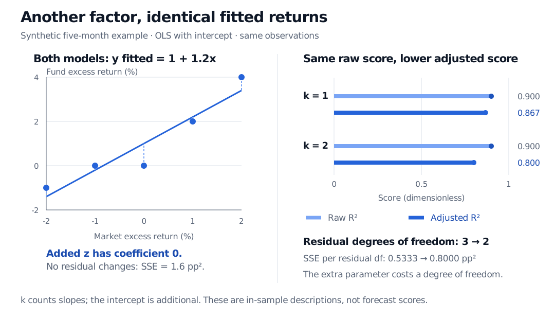
Its estimated coefficient is exactly zero. The enlarged model is still y^=1+1.2x+0z: every prediction and residual in the table stays the same. Raw R-squared remains 0.9, but residual degrees of freedom fall from 3 to 2:
Rˉk=22=1−16/41.6/2=0.8.
Synthetic five-month factor example: both OLS models fit fund excess return as 1 plus 1.2 times market excess return. Adding a linearly independent factor column with coefficient zero leaves raw R-squared at 0.900 but lowers adjusted R-squared from 0.867 to 0.800 as residual degrees of freedom fall from 3 to 2.
Original synthetic example. Returns are in percent; residual differences are percentage points. Both fits use the same five rows and an intercept. The added factor changes the parameter count, not the fitted line.
The adjusted score falls because 1.6/2=0.8pp2 exceeds 1.6/3≈0.5333pp2. It is a worse error estimate per residual degree of freedom. Saying the extra factor “explains nothing in this sample” is justified here; saying it can never matter in another sample is not.
How much improvement earns another parameter?
For nested, full-rank, unpenalised OLS models fitted to the same response on exactly the same rows, adding predictors cannot increase the minimum SSE: the larger model can reproduce the smaller fit by setting the added coefficients to zero. That is why raw R-squared cannot fall. This argument fails if adding a predictor also drops observations with missing data.
Adjusted R-squared rises precisely when the reduction in SSE outweighs the reduction in residual degrees of freedom. In the example, a two-factor model would need
2SSEnew<31.6⟺SSEnew<1516≈1.0667pp2.
A small SSE reduction is therefore insufficient. Conversely, the rule is fairly permissive: when adding one independent predictor and the larger model has positive SSE, adjusted R-squared increases exactly when the usual partial F-statistic exceeds 1. That algebraic threshold is not a conventional statistical-significance test. Its interpretation as an exact F-test needs additional error assumptions, and a chosen significance level usually imposes a stricter threshold. Repeatedly searching factors until the score improves also introduces overfitting.
For the matrix formulation and nested-model comparison, Multiple Linear Regression supplies the full-rank setup and partial F-test (public preview; full lesson requires membership).
Read the score within its limits
Negative values are possible. If SSE/(n−k−1)>SST/(n−1), adjusted R-squared is negative. This means the degrees-of-freedom-adjusted residual variation exceeds the sample response variance; it does not mean a negative fraction of raw variation was explained. Do not clip the result to zero.
The usual upper bound is 1, and adjusted R-squared is at most raw R-squared. They coincide for a perfect fit, provided the response varies and residual degrees of freedom remain positive. An intercept-only model has both scores zero for a nonconstant response.
Undefined is different from poor. A constant response gives SST=0; a saturated model has no positive residual degrees of freedom. The displayed formula supplies no valid score in either case. Rank-deficient designs require a rank-aware parameter count rather than counting duplicated columns as new parameters.
The intercept convention matters. Software may use an uncentred total sum of squares and a different adjustment when the intercept is omitted. Check the reported definition before comparing it with the centred formula here. The same parameter-count rule should not be transferred mechanically to ridge, lasso or other penalised fits.
Compare like with like. Keep the response, rows and fitting convention fixed. Scores for a return regression and a log-price regression do not provide a clean model ranking. Changing the sample period changes the task as well as the score.
Adjusted R-squared is an in-sample fit criterion, not a held-out score, causal claim, or guarantee of an optimal forecast. A contemporaneous factor model can describe exposure without predicting returns available to trade. Forecast evaluation needs predictors available at the forecast origin and a suitable time-ordered holdout or cross-validation design. Residual structure still matters: Regression Assumptions and Diagnostics explains why dependence, changing volatility and misspecification survive a good fit statistic (public preview; full lesson requires membership).
Sources
Chris Brooks, Introductory Econometrics for Finance, 2nd ed., Cambridge University Press, 2008, §3.8.3, “Adjusted R²,” and §3.10 on non-nested model comparison. The book's parameter count includes the intercept; this article's k counts slopes only.