Use the regression F-test to judge a group of coefficient restrictions: compare nested fits, count degrees of freedom and interpret the exact null tail.
F-test
An F-test is a hypothesis test whose statistic is compared with an F-distribution under the null model. In regression, it asks whether imposing a set of coefficient restrictions worsens the fit by more than the model's noise can plausibly explain. This lets a quant test a proposed group of factors together, rather than judge each coefficient separately.
The name covers several tests. The nested-regression test below compares two fits to the same response on the same observations. A test comparing two population variances also uses an F reference distribution, but answers a different question.
Two new factors have to earn their place together
Suppose a researcher considers adding size and value factors to a market-factor model of a fund's monthly excess return. Before looking at the result, the researcher specifies the null hypothesis: both additional coefficients are zero.
The restricted model keeps the intercept and market coefficient free. It is nested inside the unrestricted model: setting the size and value coefficients to zero reproduces it exactly. The alternative is that at least one of those two coefficients is nonzero, conditional on the market factor already being included.
Here is an original synthetic summary, with excess returns measured in percentage points (pp). Both models are fitted by ordinary least squares to the same 30 rows. These numbers illustrate the calculation; they are not observations from a particular fund.
Fit
Free coefficients, including intercept
Residual sum of squares, pp²
Restricted: market only
2
120
Unrestricted: market, size and value
4
84
The residual sum of squares (RSS) is the sum of squared differences between observed and fitted responses. It falls by 36 pp², or 30% of the restricted RSS. That looks substantial, but a larger nested OLS model can always fit at least as well: it could simply set the new coefficients to zero. A lower RSS alone is not evidence that the additions matter in the population.
Price the improvement in units of residual noise
Let kR and kU count the restricted and unrestricted free coefficients, including any intercept. Let q=kU−kR be the number of independent restrictions. For this nested comparison,
F=RSSU/(n−kU)(RSSR−RSSU)/q.
The numerator is improvement per restriction relaxed. The denominator estimates the error variance from the unrestricted fit; it is not the restricted model's residual mean square. The two quantities have the same squared-response units, so their ratio is unitless.
In the example, q=2 and the unrestricted residual degrees of freedom are 30−4=26. Hence
F=84/26(120−84)/2=42/1318=739≈5.5714.
The improvement per added coefficient is about 5.57 times the unrestricted residual variance estimate. We still need a null distribution to judge how unusual that is.
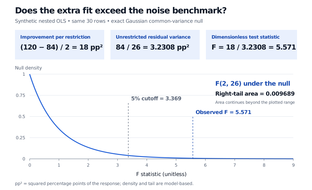
Synthetic same-sample nested regression comparison: improvement per restriction is 18 squared percentage points, residual variance estimate is 84 divided by 26, and F is 5.571. Under F with 2 and 26 degrees of freedom, the right-tail probability is 0.009689 and the 5 percent cutoff is 3.369.
Original synthetic illustration. The curve is the exact F(2, 26) null density under the stated Gaussian common-variance model; the shaded right tail continues beyond the displayed range. pp² denotes squared percentage points, not a percentage return.
Where the exact reference law comes from
For the usual finite-sample result, take the unrestricted design matrix X as fixed and full column rank, with n>kU. Assume the unrestricted conditional mean is correctly specified and
y=Xβ+ε,ε∼N(0,σ2In),σ2>0.
These are independent Gaussian errors with a common variance. The restrictions must be specified independently of the realised response used for the test. Under the null, least-squares geometry separates the extra fit and the remaining residual into orthogonal Gaussian components. Consequently,
σ2RSSR−RSSU∼χq2,σ2RSSU∼χn−kU2,
and these two quantities are independent. Dividing each by its degrees of freedom gives F∼Fq,n−kU. The unknown error variance cancels. This is why both degrees of freedom matter, and why the difference in RSS is used rather than the raw ratio RSSR/RSSU.
For the example, the p-value is the upper-tail probability
p=P(F2,26≥739)=0.0096889010407.
The closed-form survival function in this particular case is P(F2,26≥x)=(1+x/13)−13 for x≥0, so the tail is exactly 0.713. At a prespecified 5% significance level, reject the joint zero-coefficient null. This is evidence against the pair of restrictions under the model, not a 99.03% probability that the added factors are useful.
The Multiple Linear Regression lesson develops the projection setup, partial F-test and the role of correlated predictors. Its outline is public; the full lesson requires membership.
What a rejection leaves unanswered
A joint rejection does not establish that both factors matter individually. It says that the restrictions cannot jointly be maintained at the chosen level under the model. Separate coefficient questions need their own tests, and searching many possible factor groups changes the interpretation of a selected p-value.
Nor does rejection establish causation, profitable trading or improved forecasting on new data. A factor can explain historical return variation without supplying a tradable forecast. Economic magnitudes, costs and out-of-sample evaluation remain separate work.
Check the comparison before calculating it. Dropping rows because an added predictor is missing changes the sample; comparing RSS from the two resulting samples is invalid. Comparing a regression of returns with one of log returns changes the response. Two nonnested models cannot be put into this formula merely because one has more coefficients. Regularised fits also do not automatically satisfy the OLS calculation.
The exact error assumptions matter in finance. Heteroskedasticity or autocorrelation breaks the spherical Gaussian derivation. A covariance-robust Wald test, with an appropriate heteroskedasticity, time-series or cluster covariance estimator and justified asymptotics, may address a related joint hypothesis. Relabelling the classical RSS statistic “robust F” does not provide that protection.
If both RSS values are equal and positive, this statistic is zero and its upper-tail p-value is one. If the unrestricted RSS is zero, the variance estimate vanishes; the ordinary ratio cannot be reported as a finite F statistic. These boundary cases should be handled explicitly.
The other F-tests you will meet
The global regression F-test is the nested comparison against an intercept-only model: all slopes are restricted to zero. In a one-way ANOVA, group indicators form the regressors and equality of the group means is the restriction. Both fit the same extra-sum-of-squares logic.
With one independent linear restriction, the classical F statistic equals the square of the corresponding Student t statistic, using the same unrestricted variance estimate. Its upper-tail test agrees with the two-sided t-test; squaring removes the direction needed for a one-sided alternative.
The two-variance F-test instead uses s12/s22 to test equality of population variances from independent normal samples, with degrees of freedom n1−1 and n2−1. Its tail choice depends on the alternative. It is not a test that the regression's constant-variance assumption is automatically satisfied, and its own normality sensitivity matters. NIST's account distinguishes the one-sided and two-sided versions.
Sources
Chris Brooks, Introductory Econometrics for Finance, 2nd edition, Cambridge University Press (2008), §3.4, especially equation (3.20), and §3.4.1.
John A. Rice, Mathematical Statistics and Data Analysis, 3rd edition, Duxbury (2007), §§14.4.3–14.4.5: residual variance, Gaussian coefficient inference and the least-squares projection framework.
G. Simon, Partial F Test, NYU Stern (2010), pp. 1–3: nesting, parameter restrictions and the unrestricted residual mean square.