A null hypothesis specifies a claim to test, not necessarily zero or no effect. An exact order-fill example separates the benchmark, reference law and non-rejection.
Null hypothesis
A null hypothesis, written H0, is the claim about a population or data-generating process that a hypothesis test is designed to challenge. It specifies a reference against which the observed data are assessed. The null need not mean “zero,” “no effect” or “no difference”: an execution desk can test a fill probability of 60%.
Choosing the null determines which mistaken rejection the test controls. For a quant, this makes it part of the research question, alongside the population, sampling assumptions and competing claim—not a label added after seeing the backtest.
A benchmark is a claim about the process
Suppose an execution desk asks whether a routing policy's fill probability has fallen below a stipulated benchmark. Before collecting the sample, define a fill as complete execution within a fixed time window. Select 20 comparable orders and model their fill indicators as independent, identically distributed Bernoulli trials, each with unknown success probability p.
This is a synthetic teaching model. Comparable order size, instrument and market conditions matter; shared liquidity shocks or changing conditions can break its assumptions. The 60% benchmark is stipulated, not estimated from another uncertain sample.
Under this null and the sampling model, the total fill count K has the binomial distribution:
K∼Binomial(20,0.6).
The claim p=0.6 is the null hypothesis; this distribution of the random count is its null sampling law. The observed count is neither of those things.
Now observe eight fills. The sample proportion is 8/20=0.4, below the benchmark. Because the alternative points downwards, smaller counts are more extreme. The exact one-sided p-value includes the observed count:
Pp=0.6(K≤8)=k=0∑8(k20)(0.6)k(0.4)20−k≈0.05653.
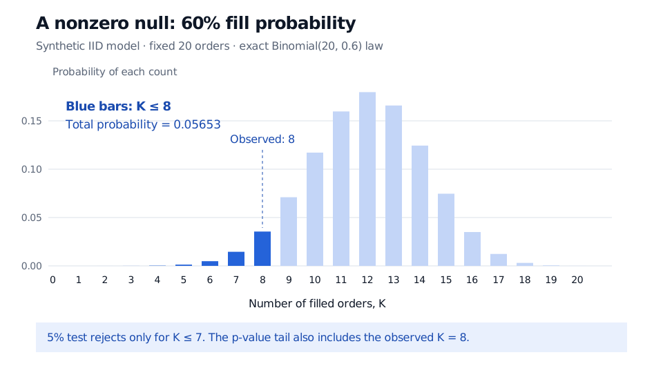
Under the benchmark model, about 5.65% of fixed samples of 20 orders would produce eight or fewer fills. At a predeclared significance level of 5%, this test does not reject the benchmark.
Exact Binomial(20, 0.6) count law. Blue bars cover zero through eight fills, with total probability 0.05653. Eight is observed; the nonrandomized 5% test rejects only at seven fills or fewer.
Original synthetic calculation. The blue bars show the observed p-value tail, not the fixed rejection region. Counts of seven or fewer have null probability about 2.10%; including eight would exceed 5%.
The gap between 2.10% and 5% comes from discrete counts. A nonrandomized exact test need not use its entire significance allowance. No normal approximation is needed here; SAS's exact binomial documentation describes the corresponding tail calculations.
A null can contain many parameter values
More generally, write H0:θ∈Θ0: the null identifies an allowed set of parameter values within a model. A simple hypothesis fully specifies the data distribution; a composite hypothesis leaves more than one possible distribution. The sampling assumptions are essential: fixing a mean alone does not generally specify a whole distribution.
For the desk's question, the exhaustive one-sided formulation is
H0:p≥0.6,H1:p<0.6.
This composite null says the fill probability meets or exceeds the benchmark. For this lower-tail test, its worst-case null probability is attained at the boundary:
p∈[0.6,1]supPp(K≤8)=P0.6(K≤8).
Why? Increasing the fill probability shifts counts upwards, making a low count less likely. One can generate each fill by comparing the same independent uniform draw with p: increasing p can only add fills. Thus the boundary 0.6 is least favourable for false rejection, and the same p-value remains valid over this entire null set. Boundary evaluation is justified by this model and ordering; it is not a universal recipe for composite tests.
What non-rejection leaves open
“Did not reject 60%” does not mean “confirmed 60%.” Eight fills remain an estimate below the benchmark, and a short sample can miss a genuine deterioration. Statistical power describes the chance of detecting a specified departure under a chosen test.
Nor has the desk established equivalence to the benchmark. That requires defining an acceptable tolerance in advance and using a procedure designed to establish that the deviation is sufficiently small. Ordinary non-rejection does not supply that evidence.
Finally, 0.05653 is not the probability that H0 is true, and its complement is not the probability of deterioration. A posterior probability requires a Bayesian model and prior information. The ASA's statement distinguishes null-model tail probabilities from probabilities assigned to hypotheses and cautions against basing business decisions on a threshold alone.
To study the general testing framework beyond this count example, Confidence Intervals and Hypothesis Testing develops parameter-set hypotheses, test errors and normal-mean tests. Its public page is a preview; the full lesson requires membership.
Sources
John A. Rice, Mathematical Statistics and Data Analysis, 3rd edition (2007), §§9.2–9.2.2: null and alternative hypotheses, simple and composite claims, significance levels and p-values.