Alternative hypothesis: Definition & Examples

An alternative hypothesis, written

H_1

H_a

, specifies the population parameter values a statistical test is designed to detect in opposition to the null hypothesis. It is a claim about the data-generating process, not a description of the sample already observed.

For a trading strategy, “the expected net return is positive” is an alternative hypothesis. “The backtest made money” is an observed result. A profitable sample can occur even when the strategy's true expected return is zero or negative.

Write the claim before examining the returns

Let

\mu

be a strategy's expected return per fixed observation period, after a specified cost model. A desk interested specifically in positive expected net returns can predeclare

H_0:\mu\le 0 \qquad\text{versus}\qquad H_1:\mu>0.

The alternative is the set of all positive population means, not one particular target return. Both hypotheses here are composite: each allows many parameter values. The boundary

\mu=0

belongs to the null. Negative true means belong there too; they do not establish the positive-return claim.

The wording determines which departures count as evidence. These are different questions:

Research question	Null	Alternative
Is expected net return positive?	$\mu\le0$	$\mu>0$
Is expected net return negative?	$\mu\ge0$	$\mu<0$
Does expected net return differ from zero?	$\mu=0$	$\mu\ne0$

The first two are one-sided. The third is two-sided: sufficiently large departures in either direction count. Choose the question, observation horizon, sample size and testing rule before using the evaluation data. A negative outcome in the positive-return test is not permission to switch to the negative-return alternative afterward.

A positive estimate still needs a threshold

Consider a hypothetical, fixed-sample experiment, not a market calibration. Assume 64 independent, identically distributed normal net returns, with population standard deviation known to be 1 percentage point per observation. The desk has predeclared the positive-return alternative above and a 5% significance level.

The observed sample mean is 0.25 percentage points. Its standard error is

\mathrm{SE}=\frac{1}{\sqrt{64}}=0.125 \quad\text{percentage points}.

At the null boundary, the standardised test statistic has a standard normal distribution:

Z=\frac{\bar X-0}{\sigma/\sqrt n}, \qquad z_{\mathrm{obs}}=\frac{0.25}{0.125}=2.

Writing

\Phi

for the standard normal cumulative distribution function, the fixed rule rejects when

Z>\Phi^{-1}(0.95)=1.644854

, equivalently when the sample mean exceeds 0.205607 percentage points. The observed 0.25 clears that threshold. The right-tail p-value is

p=1-\Phi(2)\approx0.02275<0.05.

Thus the test rejects the nonpositive-mean null at the chosen level, providing evidence for the positive-mean alternative under the stipulated model. It does not assign a 97.725% probability to $H_1$ or guarantee future profitability.

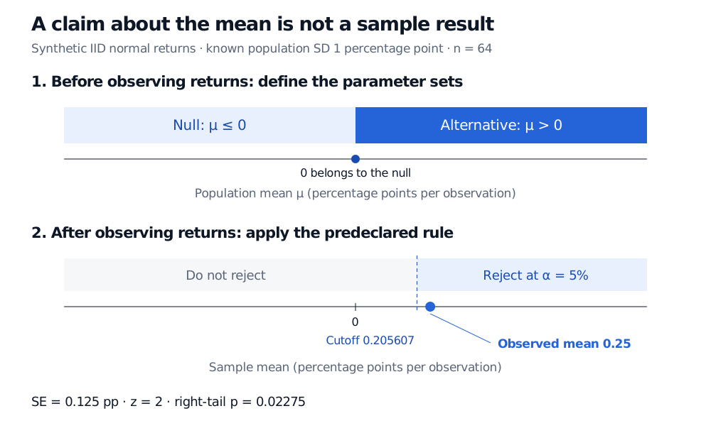
Two separate axes distinguish a predeclared parameter claim from a sample decision. The null contains population means at or below zero and the alternative all positive means. For 64 IID normal returns with known SD 1 percentage point, the observed sample mean 0.25 exceeds the 5% right-tailed cutoff 0.205607; standard error is 0.125 and z is 2.

Original hypothetical example. Both axes use percentage points per observation. The upper axis classifies population means; the lower axis applies the fixed test to a sample mean. A positive sample mean alone need not fall in the rejection region.

Why calculate the cutoff at zero when the null includes every negative mean? For a fixed sample-mean cutoff $c$ ,

\mathbb P_\mu(\bar X>c) =1-\Phi\left(\frac{c-\mu}{0.125}\right)

increases with $\mu$ . Its largest value over $\mu\le0$ therefore occurs at zero. With the chosen cutoff this maximum is 5%; the rejection probability is smaller at every negative true mean. This monotonicity is what makes boundary calibration control the entire composite null.

The alternative also defines what the test can miss

A test can fail to reject even when

H_1

is true. Its statistical power depends on the particular true mean within the alternative: a tiny positive mean is harder to distinguish from zero than a large one. “There was no significant result” does not prove the population mean is nonpositive.

Nor does statistical evidence decide the relevant economic hurdle. If the desk requires a minimum expected return $h$ , the meaningful question may instead be $H_0:\mu\le h$ versus $H_1:\mu>h$ . Specify that hurdle and the cost convention in advance.

The example's exact normal calculation depends on normal, independent observations and a genuinely known population SD. Estimating SD from the same normal sample leads to Student's $t$ inference; serial dependence requires an appropriate sampling-variance model. Testing many candidate strategies or repeatedly checking accumulating data also changes the error-control problem.

For the sampling-distribution machinery and the connection to confidence intervals, continue with Confidence Intervals and Hypothesis Testing (public preview; full lesson requires membership).

Sources

Casella, G. and Berger, R. L., Statistical Inference, 2nd edition, §8.1, Definitions 8.1.1–8.1.3: hypotheses as statements about population parameters, complementary parameter sets and rejection regions.
NIST/SEMATECH e-Handbook, §7.2.2: Testing a single population mean: directional hypotheses and the known-SD normal statistic.
University of Wisconsin–Madison, Statistics 571: Significance Tests with Known Standard Deviation: one-sided versus two-sided questions and choosing the direction before inspecting data.

Write the claim before examining the returns

A positive estimate still needs a threshold

The alternative also defines what the test can miss

Sources

Related terms

Expected return

Null hypothesis

P-value

Standard error

Statistical power

Test statistic