Standard error measures how an estimator varies across samples. Separate it from outcome volatility, calculate a mean SE, and see how dependence and sampling units change the calculation.
Standard error
The standard error of an estimator is the standard deviation of its sampling distribution: how much that estimator varies across repetitions of the specified data-generating and sampling process. It measures uncertainty in an estimate, such as a strategy's mean P&L, rather than the dispersion of individual P&L outcomes.
For an estimator θ^ with finite variance,
SE(θ^)=Var(θ^).
That variance is usually unknown. The number reported by software is then an estimated standard error, written here as SE(θ^). A standard error is neither the realised error θ^−θ nor a bound on it. It also does not account for bias: a systematically wrong estimate can have a small SE. Wasserman distinguishes the sampling standard deviation from its estimate in All of Statistics, §6.3.1.
Four P&L observations, two different spreads
Suppose a researcher records four hypothetical one-period P&Ls, in USD, from the same fixed strategy and position size:
x=(1,2,3,4),xˉ=2.5.
For this calculation, model the observations as independent and identically distributed (iid), with finite variance. These are assumptions about how the data arose; four observations cannot establish them.
The deviations from the mean are (−1.5,−0.5,0.5,1.5). Their squared sum is 5 USD2, so the sample variance, using the divisor n−1, is
s2=35 USD2,s=35≈1.290994 USD.
This sample standard deviation estimates the dispersion of one period's P&L. For the sample mean, the estimated standard error is instead
SE(Xˉ)=4s=125≈0.645497 USD.
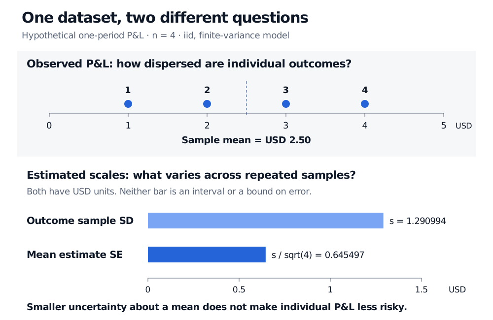
It estimates the spread of the four-observation mean across repeated samples of four. Averaging can make the mean estimate less variable without making the next individual outcome safer. Reporting USD 0.645497 as the strategy's one-period P&L volatility would answer the wrong question.
Four hypothetical independent P&L observations are USD 1, 2, 3 and 4, with sample mean USD 2.50. Outcome sample SD is USD 1.290994; estimated SE of the four-observation mean is USD 0.645497. Bars compare scales, not confidence intervals.
Original hypothetical example under an iid finite-variance model. Both scales are in USD; neither bar is a confidence interval or an error bound.
Why divide by the square root of the sample size?
Let the iid observations have population mean μ and variance σ2. Independence eliminates cross-covariances, giving
Var(Xˉ)=n21i=1∑nVar(Xi)=nσ2,SE(Xˉ)=nσ.
Replacing the unknown σ with s gives the estimated SE. Normality is not needed for this variance identity. It matters when choosing a distribution for inference. The University of Michigan notes on standard errors distinguish the iid mean formula from its plug-in estimate.
Under this same fixed-distribution model, quadrupling the sample size halves the true SE of the mean. The calculation is not a universal rule for all estimators, dependent data or changing market regimes. An estimated SE can even rise when new observations reveal more dispersion than the original sample suggested.
Count information, not just rows
Without independence, the general finite-variance identity is
Var(Xˉ)=n21(i=1∑nVar(Xi)+2i<j∑Cov(Xi,Xj)).
Positive cross-covariances raise the variance relative to the same marginal variances with zero covariance. Negative cross-covariances can lower it. Ignoring serial correlation in a return history therefore changes the uncertainty calculation, not merely the wording of a caveat.
For a separate model illustration, suppose four observations each have known variance 4 USD2 and every distinct pair has known correlation ρ=0.5. These parameters are stipulated, not estimated from the four P&Ls above. With equal variances and pairwise correlation,
Var(Xˉ)=nσ2[1+(n−1)ρ]=44(1+3×0.5)=2.5 USD2.
The SE is 2.5≈1.581139 USD, compared with USD 1 under independence. The observation count is unchanged; their joint information is different.
Heteroskedasticity means variances differ, or conditional variances change. With independent observations, the variance of the mean is ∑iσi2/n2; heteroskedasticity alone does not create cross-covariances or automatically inflate every SE. In regression, conventional coefficient SE formulas may nevertheless fail under heteroskedastic errors. Heteroskedasticity-consistent errors address that issue; time-series dependence may require Newey–West standard errors or another justified dependence-aware method. These procedures have their own assumptions and sample-size limitations; they do not repair a misspecified economic model. Brooks discusses the distinction in §4.5.7 of Introductory Econometrics for Finance (2nd ed.).
The sampling unit must match the claim. A hundred trades placed on the same market move are not necessarily a hundred independent replications. Comparing two strategies on matching dates calls for analysing their paired differences, including their covariance. Overlapping holding periods share returns; many instruments observed on one date may share a common shock. Depending on the design, uncertainty may need to be organised by date, cluster or time block rather than by individual row. Merely duplicating rows adds no independent information.
Without that normal model, four observations do not justify a normal approximation simply because an SE can be calculated. Heavy tails, rare losses and dependence can make a short track record particularly misleading. The SE itself is estimated imprecisely, and if the relevant variance is infinite, a finite population standard error need not exist. A positive average with a small reported SE also says nothing by itself about costs, selection of the strategy after seeing the data, or future stability.
For a first calculation of sample summaries and their assumptions, read Basic Statistics and Regression, available in full with a free signed-in account. For the move from an SE to normal-family pivots, intervals and tests, see Confidence Intervals and Hypothesis Testing, whose full lesson requires membership and has a public preview.
Sources
Larry Wasserman, All of Statistics: A Concise Course in Statistical Inference, §6.3.1, equation (6.5), and Example 7.10: standard error as sampling standard deviation; the mean and its estimated SE.
Chris Brooks, Introductory Econometrics for Finance, 2nd ed., §4.5.7, pp. 152–153: heteroskedasticity corrections versus heteroskedasticity-and-autocorrelation-consistent errors.