Compute sample standard deviation, track percentage-point units, and distinguish observation dispersion from mean standard error and uncertainty in estimated volatility.
Sample standard deviation
The sample standard deviation is the nonnegative square root of the usual sample variance. It measures how dispersed observed values are around their sample mean, in the original data units. For a sample of n≥2 finite observations,
xˉ=n1i=1∑nxi,s=n−11i=1∑n(xi−xˉ)2.
The square root converts the squared units of sample variance back to the units of each observation. A return SD can therefore be compared with a return; a variance cannot. The calculation itself needs no normality or independence assumption. Such assumptions enter when interpreting s as an estimate of a population's standard deviation, or assessing its uncertainty.
Five returns, three numbers worth keeping separate
A researcher checks five synthetic one-day simple returns on one strategy: −2%, −1%, 0%, +1% and +2%. Express the observations in percentage points (pp), so a 1% return is recorded as 1, rather than 0.01.
Observation
Return (pp)
Deviation from mean (pp)
Squared deviation (pp²)
1
−2
−2
4
2
−1
−1
1
3
0
0
0
4
1
1
1
5
2
2
4
The sample mean is zero, and the centred squares sum to 10 pp2. Thus
s2=5−110=2.5 pp2,s=2.5≈1.5811 pp.
This is a measure of dispersion around the observed mean. It is not a maximum possible daily loss or a claim that a fixed proportion of returns lies within one SD. Squaring gives large deviations extra weight, so one extreme observation can materially change the estimate. Whether an outlier is a data error or a real risk event needs investigation before deletion.
Now change the statistical question:
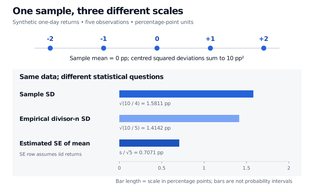
Describe only these five observations as an empirical population. Give each record probability 1/5. Its divisor-n variance is 10/5=2 pp2, and its SD is 2≈1.4142 pp. This is a valid descriptive convention, distinct from the usual divisor-n−1 sample SD.
Estimate uncertainty in the mean of an iid return model. If the observations are independent draws from the same finite-variance distribution, the estimated standard error of the sample mean is s/n=0.5≈0.7071 pp. That number concerns the average across hypothetical repeated samples, rather than the spread of individual returns.
Five synthetic daily returns are −2, −1, 0, 1 and 2 percentage points. Sample SD is 1.5811 pp, empirical divisor-n SD is 1.4142 pp, and the estimated iid mean standard error is 0.7071 pp.
Original synthetic one-day example. The bars compare numerical scales in percentage points; they are not probability intervals. Only the mean-SE row invokes an iid sampling model.
The last number is also not the standard error of the estimated volatilitys. Uncertainty about a mean and uncertainty about a standard deviation are different estimation problems. Five observations provide little evidence about the stability or tails of a strategy's return distribution, even when the arithmetic is exact.
What the correction fixes—and what it does not
After subtracting the fitted mean, the deviations sum to zero. Only n−1 deviations can vary freely. For iid observations with finite population variance σ2, the expected centred sum of squares is (n−1)σ2. Dividing by n−1 therefore makes the random statistic S2 an unbiased estimator of that variance:
E[S2]=σ2.
Taking a square root does not preserve unbiasedness. An exact small example shows why. Draw two independent observations, each equal to −1 pp or +1 pp with equal probability. The population SD is 1 pp. Half the samples have matching signs and give S=0; half have opposite signs and give S=2 pp. Consequently,
E[S2]=1 pp2,E[S]=22 pp≈0.7071 pp<1 pp.
The sample variance is unbiased; the sample SD is not. More generally, concavity of the square root gives E[S]≤E[S2]=σ under this iid finite-variance setup. The correction concerns averages over repeated samples, not a promise that any single estimate equals the true risk. Dependence or selective data collection requires separate reasoning.
Units, horizon and software conventions
If the original returns are stored as decimals, the same five numbers are −0.02, −0.01, 0, 0.01 and 0.02. The sample variance is then 0.00025 in squared decimal-return units, and
s=0.0158113883 in decimal-return units=1.58113883 pp.
Variance scales by the square of the conversion factor; SD scales by its absolute value. For transformed data yi=a+bxi, sy=∣b∣sx: adding a constant changes the mean but not dispersion, and reversing signs does not make SD negative. A constant sample has s=0; with fewer than two observations the divisor-n−1 statistic is undefined.
A report should name the return definition, observation interval, window, units and divisor. Software conventions differ, so verify the divisor rather than inferring it from a function's name.
Calling a return SD historical volatility still leaves the horizon explicit. Multiplying daily SD by a square root of an annual observation count requires an aggregation model: variance adds for uncorrelated additive increments with a common variance. Log returns add through time; simple returns compound. Serial covariances, changing volatility and overlapping intervals can alter the calculation. The five-day sample here supplies no automatic annualised figure and no forecast guarantee.
For the calculation alongside other basic summaries, see Basic Statistics and Regression (full lesson free with a signed-in account). For the return-definition and dependence issues behind a volatility interpretation, see Financial Return Characteristics (public preview; full lesson requires membership).
Sources
John A. Rice, Mathematical Statistics and Data Analysis, 3rd ed., §4.2, “Variance and Standard Deviation,” and §6.3, “The Sample Mean and the Sample Variance.” The exact chi-squared sampling result in §6.3 assumes iid normal observations.