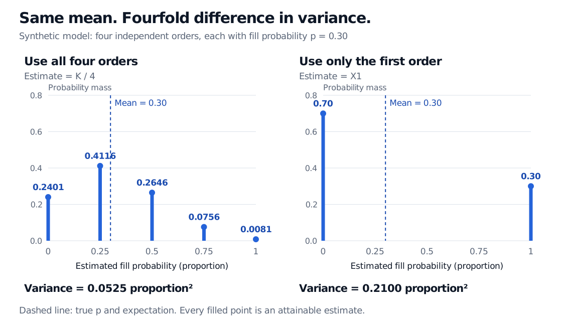
An unbiased estimator hits its target in expectation across samples. A four-order fill model shows why that can coexist with large uncertainty and no exactly correct realised estimate.
Unbiased estimator
An unbiased estimator is an estimator whose expected value equals the parameter it is trying to estimate, for every parameter value in the stated statistical model. It has zero bias. The claim concerns a procedure applied to random samples; one observed estimate can still be far from the truth.
For a trading desk estimating an order's fill probability, that distinction matters. A procedure can report the right probability on average across repeated datasets while giving a very uncertain answer from today's small dataset. Unbiasedness settles the centre of the sampling distribution, not its spread.
What the expectation is taken over
Let the data have distribution Pθ, where the unknown, fixed parameter is θ∈Θ. An estimator θ^=T(X1,…,Xn) is unbiased for θ when it is integrable and
Eθ[θ^]=θfor every θ∈Θ.
Integrable means Eθ[∣θ^∣]<∞, so the expectation is well defined and finite. The subscript records which data-generating distribution supplies the expectation. If the target is a function g(θ), the right-hand side becomes g(θ).
Imagine holding the true parameter fixed, repeatedly drawing a fresh dataset under the same sampling rules, and recalculating the estimator. Unbiasedness says the probability-weighted average of those possible estimates equals the target. It does not average over different possible true parameters. Nor does zero error at one special parameter value establish unbiasedness throughout the model: a constant estimator equal to zero hits the target when θ=0 but fails whenever θ=0.
Four orders, no exactly correct answer
Consider a synthetic execution model. Four comparable orders are submitted under the same conditions. Let Xi=1 if order i fills within a fixed horizon and Xi=0 otherwise. Assume independent Bernoulli outcomes with a common probability p∈0,1]. Define the count K=X1+⋯+X4 and estimate the fill probability by the [sample mean,
Now stipulate the true probability is p=0.30. Exact binomial probabilities give:
Fills K
Reported estimate K/4
Probability of that estimate
0
0
0.2401
1
0.25
0.4116
2
0.50
0.2646
3
0.75
0.0756
4
1
0.0081
The probabilities sum to one, and their weighted average estimate is exactly 0.30. Yet none of the possible estimates equals 0.30. Every realised estimate misses the truth, even though the estimator is unbiased. For example, a dataset containing one fill produces 0.25; that particular error does not make the procedure biased.
The count distribution and the estimator distribution use different horizontal units: a count K=2 corresponds to an estimated probability K/4=0.50. Dividing count outcomes by four also divides their variance by sixteen.
Exact synthetic sampling laws for four independent order fills with p = 0.30. K/4 takes 0, 0.25, 0.5, 0.75 or 1; X1 takes 0 or 1. Both expectations are 0.30, but variances are 0.0525 and 0.21 proportion squared. Neither estimator can realise 0.30.
Original synthetic model, exact probabilities: four IID Bernoulli fills with p=0.30. Both estimators are unbiased, but using all four orders cuts variance by a factor of four. Dashed lines mark the common expectation; filled points mark attainable estimates.
A deliberately wasteful unbiased estimator
Suppose the desk ignores the final three orders and reports p~=X1. This is also unbiased: its expectation is p. At p=0.30, it reports zero with probability 0.70 and one with probability 0.30.
Its variance, however, is four times the variance of the four-order proportion:
The displayed numerical values use p=0.30; the formulas apply throughout [0,1]. Variances have units of proportion squared. An unbiasedness label alone cannot choose between these two procedures.
For any estimator with a finite second moment, mean squared error combines dispersion and systematic displacement:
Eθ[(θ^−θ)2]=Varθ(θ^)+(Eθ[θ^]−θ)2.
For an unbiased estimator, MSE equals variance. A biased alternative can sometimes reduce variance enough to achieve lower MSE; requiring zero bias rules that alternative out before the comparison even starts. Casella and Berger's §7.3.1 develops this distinction through variance estimation.
For the likelihood connection, read Estimation and Maximum Likelihood: it derives the Bernoulli estimator and compares biased and unbiased normal-variance estimators. The public page offers a preview; the full lesson requires membership.
What the label leaves unresolved
Will more data make it accurate? That is a question about a sequence of estimators and consistency. With an IID Bernoulli sample, K/n converges in probability to p. But the procedure that always reports only X1 remains unbiased for every sample size and gains no precision. At p=0.30, its absolute error exceeds 0.20 with probability one for every n. Unbiasedness does not imply consistency.
Are the orders dependent? If their marginal fill probabilities still all equal p, their average remains unbiased. Its variance includes cross-order covariances, so the independent-trial formula need not hold. In the extreme case that all four indicators always equal the same Bernoulli variable, the four-order average is just that one variable: its variance is 0.21, with no averaging gain.
Which orders entered the dataset? Logging only filled orders, deleting failed executions, stopping after a favourable outcome, or selecting the best-looking venue after inspecting results changes the sampling procedure. The fixed-sample calculation above does not establish unbiasedness after those choices. Likewise, if fill probabilities change with queue position or market conditions, an average may target a mixture of historical probabilities rather than the probability relevant to a new order. A proof of unbiasedness is only as applicable as its target and sampling assumptions.
Sources
George Casella and Roger L. Berger, Statistical Inference, 2nd edition, §7.3.1, especially Definitions 7.3.1–7.3.2 and Examples 7.3.3–7.3.4: bias, unbiasedness and mean squared error.
UC Berkeley, Stat 135: Sampling distribution of the Mean, “The Sampling Distribution” and “Direct calculation of Mean and Variance of Estimator”: repeated samples, sample means and proportions, and the assumptions behind their variance.