Bias is an estimator’s expected error across repeated samples. See why a downward-biased variance estimate can still overestimate risk in one sample.
Bias of an estimator
The bias of an estimator is its expected value minus the parameter it is intended to estimate. It measures the direction and size of the estimator’s average error across repeated samples drawn under the same model. A risk estimate can therefore be biased downward even when the number reported for a particular sample is too high.
For a scalar parameter θ and an estimatorθ^, the definition is
Biasθ(θ^)=Eθ[θ^]−θ.
The subscript identifies the sampling model at the specified parameter value. Positive bias means an average overestimate; negative bias means an average underestimate. An unbiased estimator has zero bias at every parameter value in its stated model. Before using this definition, the expectation must exist. Bias has the same units as the parameter.
A short risk window can overestimate despite downward bias
Consider a deliberately simple model: independent, identically distributed one-period log returns, with normal distribution, true mean 1 pp and true variance σ2=4 pp2. Here pp denotes percentage-point units: 1 pp corresponds to a decimal log return of 0.01. These are synthetic assumptions, not a claim that observed market returns are iid normal.
A researcher estimates variance from four returns, using the fitted sample mean Xˉ. Compare the two rules
Vn=n1i=1∑n(Xi−Xˉ)2,S2=n−11i=1∑n(Xi−Xˉ)2.
S2 is the usual bias-corrected sample variance. With n=4, their repeated-sample expectations and one illustrative result are:
Quantity
Divide by n: Vn
Divide by n−1: S2
Expected estimate
3 pp2
4 pp2
Bias relative to true variance 4
−1 pp2
0 pp2
Estimate from returns −2,0,2,4 pp
5 pp2
20/3 pp2≈6.67 pp2
For that sample, the mean is 1 pp and the squared deviations sum to 9+1+1+9=20 pp2. Dividing by four gives five. The negatively biased estimator has overestimated the true variance by 1 pp2, or 25%. Its expected bias is instead −1 pp2, or −25% of truth. The two signs describe different objects.
Multiplying by n/(n−1) removes the expected bias, but in this sample it pushes the estimate further above the truth. Bias correction does not promise a more accurate number in every realised sample.
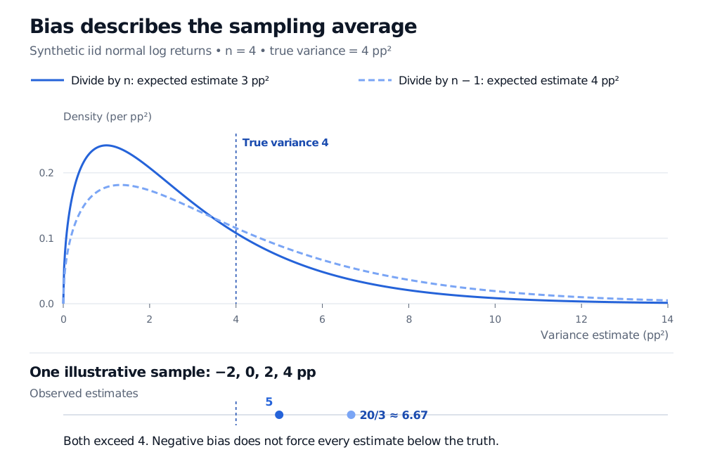
Exact sampling densities in a synthetic iid normal model with four returns and true variance 4 pp squared. The divisor-n estimator averages 3 pp squared but one sample gives 5; the divisor-(n minus 1) estimator averages 4 but that sample gives 20/3, approximately 6.67. Both realised estimates exceed truth.
Original analytical sampling densities, not a histogram of market returns. Returns are in percentage-point units; variance estimates are in pp². The illustrative sample is −2, 0, 2, 4 pp. The lower strip uses the same horizontal scale.
The figure shows the sampling distributions, rather than the distribution of individual returns. Under the normal model, nVn/σ2=(n−1)S2/σ2 has a chi-squared distribution with n−1 degrees of freedom. The curve’s peak is its mode; bias depends on its mean, which need not coincide with that peak.
Why fitting the mean changes the divisor
The source of the bias is visible without normality. For iid observations with finite variance and n≥2,
i=1∑n(Xi−Xˉ)2=i=1∑n(Xi−μ)2−n(Xˉ−μ)2.
Taking expectations subtracts nVar(Xˉ)=σ2 from nσ2, leaving (n−1)σ2. Hence
E[Vn]=nn−1σ2,Bias(Vn)=−nσ2,E[S2]=σ2.
Fitting the centre to the same observations reduces their squared deviations on average. Dividing by n−1 compensates for this specific effect. If the population mean μ were known and used instead, n−1∑i(Xi−μ)2 would already be unbiased. Conversely, the familiar correction alone does not establish unbiasedness for serially dependent returns or a time-varying variance target.
The correction concerns variance. Taking S=S2 does not generally produce an unbiased estimator of standard deviation: the square-root transformation changes the expectation. Under the nondegenerate normal model above, concavity gives E[S]<σ.
Zero bias is one criterion
With finite second moments, mean squared error combines sampling spread and squared bias:
Eθ[(θ^−θ)2]=Varθ(θ^)+Biasθ(θ^)2.
In the four-observation normal example, Vn has variance 6 pp4 and squared bias 1 pp4, so its MSE is 7 pp4. The unbiased S2 has MSE 32/3 pp4≈10.67 pp4. The biased rule wins under squared-error loss. That does not determine which rule is preferable when underestimating risk is more costly than overestimating it. Berkeley’s treatment explains this bias–variance comparison.
Finite-sample bias also differs from consistency. Here −σ2/n tends to zero, and Vn is consistent under iid sampling with finite variance. In general, vanishing bias alone does not prove consistency: the remaining sampling error must also concentrate.