Sample variance: Definition & Examples

Sample variance measures the spread of observations around their sample mean using squared deviations. The usual convention, for a sample of at least two numbers, is

s^2=\frac{1}{n-1}\sum_{i=1}^n(x_i-\bar{x})^2, \qquad \bar{x}=\frac{1}{n}\sum_{i=1}^n x_i.

It is a number you can calculate from recorded returns without assuming a probability model. Calling it an unbiased estimate of population variance adds a claim about how the observations were generated. That distinction explains both the divisor

n-1

and its limits.

Five returns, one numerator, two questions

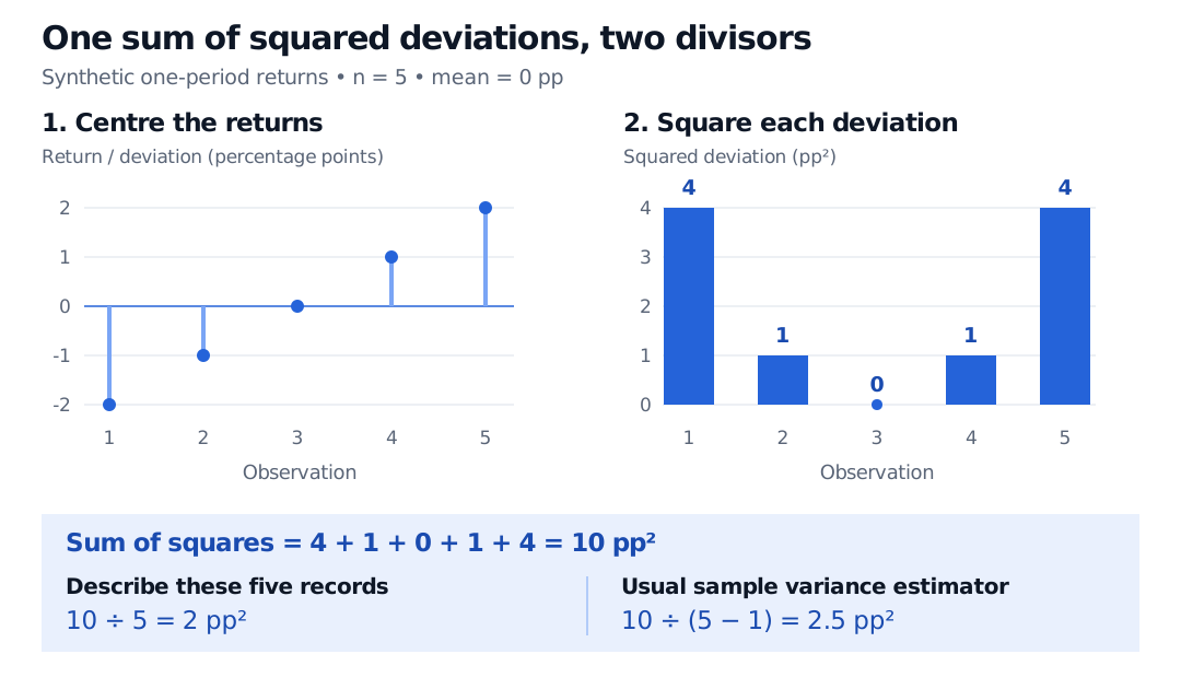
A researcher records five hypothetical, same-horizon strategy returns: −2%, −1%, 0%, 1%, 2%. In percentage-point units, the data are

(-2,-1,0,1,2)

and their mean is zero. The sum of squared deviations is

\sum_{i=1}^5(x_i-\bar{x})^2=4+1+0+1+4=10\text{ pp}^2.

Two different questions give two legitimate summaries:

Question	Calculation	Result
What is the variance of the empirical distribution, assigning probability $1/5$ to each record?	$10/5$	$2\text{ pp}^2$
What is the usual sample-variance estimate for the process generating the returns?	$10/(5-1)$	$2.5\text{ pp}^2$

The first calculation completely describes these five equally weighted records. The second uses the conventional correction for estimating an unknown mean from the same observations. It does not establish that the future return process actually has variance $2.5\text{ pp}^2$ .

Synthetic one-period returns of minus two, minus one, zero, one and two percentage points have mean zero. Their squared deviations are four, one, zero, one and four, summing to ten squared percentage points. Dividing by five gives two; dividing by four gives sample variance two point five.

Original synthetic example. Squaring removes the sign and gives larger deviations more weight. The same numerator produces different summaries when the denominator changes.

Units are squared. Expressing the returns as decimals gives

(-0.02,-0.01,0,0.01,0.02)

and

s^2=0.00025

in decimal-return-squared units. The numerical variance falls by

100^2=10{,}000

when moving from percentage points to decimal returns. Variance is not “2.5%”; taking the square root gives the sample standard deviation, here about 1.5811 percentage points.

Where the missing degree of freedom goes

The sample mean is fitted to the data. For any proposed centre $a$ , expanding the squares gives the exact identity

\sum_{i=1}^n(x_i-a)^2 = \sum_{i=1}^n(x_i-\bar{x})^2+n(\bar{x}-a)^2.

The cross term vanishes because

\sum_i(x_i-\bar{x})=0

. Thus choosing

a=\bar{x}

minimises the sum of squared deviations. Once the first

n-1

centred deviations are known, the last is forced by their zero sum. This is the one degree of freedom used to estimate the mean. Taboga's variance-estimation discussion explains the adjustment through this fitted-centre effect.

To see why the correction is exactly

n-1

, now assume

X_1,\ldots,X_n

are independent and identically distributed, with mean

\mu

and finite population variance

\sigma^2

. Uppercase

S^2

denotes the statistic before the sample is observed. Applying the identity at

a=\mu

and taking expectations,

\begin{aligned} \mathbb{E}\!\left[\sum_{i=1}^n(X_i-\bar{X})^2\right] &=n\sigma^2-n\mathbb{E}[(\bar{X}-\mu)^2]\\ &=n\sigma^2-n\frac{\sigma^2}{n}\\ &=(n-1)\sigma^2. \end{aligned}

Consequently

\mathbb{E}[S^2]=\sigma^2

S^2

is an unbiased estimator. Normality is unnecessary for this result. Dividing the same numerator by

n

instead has expectation

(n-1)\sigma^2/n

under these assumptions.

If the true mean $\mu$ were known independently, $n^{-1}\sum_i(X_i-\mu)^2$ would already be unbiased for $\sigma^2$ . Replacing that known mean with the sample mean changes the calculation, even when the observed sample mean happens to equal $\mu$ .

Unbiased does not mean correct on this sample

Consider a toy return process that takes −1 or +1 percentage point, each with probability

1/2

. Its variance is

1\text{ pp}^2

. Draw two independent returns. The four ordered samples are equally likely:

Sample, pp	$s^2$ , pp²
$(−1,−1)$	0
$(−1,+1)$	2
$(+1,−1)$	2
$(+1,+1)$	0

The average estimate across these possibilities is

(0+2+2+0)/4=1\text{ pp}^2

, exactly the population variance. Every individual estimate is nevertheless different from 1. Unbiasedness is a property of the estimator's sampling distribution, rather than a certificate for one realised value.

Taking a square root changes the estimator and its bias. In this same example, $S$ is zero or $\sqrt{2}$ with equal probabilities, so $\mathbb{E}[S]=\sqrt{2}/2\approx0.7071\text{ pp}$ , below the true standard deviation of $1\text{ pp}$ . Unbiased variance estimation does not imply unbiased standard-deviation estimation.

Before treating it as a risk estimate

With real financial observations, specify the instrument, return definition, horizon and window. Mixing daily with weekly returns changes the object being measured. A large outlier can dominate the squared deviations; deleting it can remove a genuine loss rather than repair an error. The divisor correction does not resolve that judgment.

Dependence also matters. If both observations in the toy model are always copies of the same draw, each still has marginal variance $1\text{ pp}^2$ , but $S^2$ is always zero. Selection, changing return distributions and infinite-variance models likewise require separate analysis. Merely dividing by $n-1$ does not make an arbitrary financial dataset an unbiased estimate of future risk.

A stronger result holds for iid normal observations with $\sigma^2>0$ :

\frac{(n-1)S^2}{\sigma^2}\sim\chi^2_{n-1}.

This chi-squared pivot supports exact normal-model variance intervals and tests. It is not a distribution-free result for returns. The two-point example above has a discrete sampling distribution, immediately ruling out that continuous chi-squared law.

For a calculation refresher, Basic Statistics and Regression covers variance, standard deviation and their use in regression; its full lesson is available with a free signed-in account. Estimation and Maximum Likelihood explains why a normal-model maximum-likelihood estimate uses divisor

n

and how bias differs from total estimation error; the full lesson requires membership, with a public preview.

Sources

Wasserman, L., All of Statistics: A Concise Course in Statistical Inference, Chapter 3, equations (3.9)–(3.10) and Theorem 3.17: sample moments and iid unbiasedness.
Rice, J. A., Mathematical Statistics and Data Analysis, 3rd ed., §6.3, Theorems A–B: the sample mean, sample variance and exact normal-model distribution.
Taboga, M. (2021), “Sample variance” and “Estimation of the variance”, Lectures on Probability Theory and Mathematical Statistics: divisor conventions and the effect of estimating the mean.

Five returns, one numerator, two questions

Where the missing degree of freedom goes

Unbiased does not mean correct on this sample

Before treating it as a risk estimate

Sources

Related terms

Chi-squared distribution

Outlier

Sample

Sample standard deviation

Sampling distribution

Unbiased estimator

Variance