The chi-squared distribution is the distribution of a sum of independent squared standard-normal random variables. It describes how much total squared variation a Gaussian model produces by chance. In finance, it supplies an exact reference distribution for a sample-variance statistic when observations are independent and identically distributed normal variables. That condition is part of the result, not an automatic property of daily P&L.
The parameter , pronounced “nu,” is the number of degrees of freedom. Each term is dimensionless, so is dimensionless too. Squaring removes the signs: a large negative shock contributes just as much as an equally large positive shock. The statistic measures magnitude, not direction.
The shape and the scale
The density of the central chi-squared law is
with zero probability on negative values. Here is the gamma function. Equivalently, this is a gamma distribution with shape and scale ; a rate parameterisation uses rate . This density also defines the family for any positive real , although the literal construction as squared normals requires integer .
Its mean and variance are
For example, summing four independent squared standard normals gives , with mean 4 and variance 8. These are moments of the statistic, not USD P&L moments. Since a standard normal has second moment and fourth moment , each square has variance ; independence lets the four variances add.
At low degrees of freedom the distribution is strongly right-skewed. Its boundary density diverges as for , equals at zero for , and approaches zero there for . None of these cases has an atom at zero. A density height, even an infinite limiting height, is not a point probability. These shape properties and the density formula are tabulated in the NIST distribution handbook.
Five P&L observations, four degrees of freedom
Consider an original synthetic risk-monitoring example. Before observing five one-period P&L values in USD, a team specifies an iid normal model with unknown mean and a null population variance of
The observed sample variance, calculated around the sample mean with divisor , is . The team wants an upper-sided check for increased variance.
Under the null model, the exact sampling distribution is
The USD-squared units cancel. The statistic is 8, not “USD 8” or “8 USD-squared.” The degrees of freedom are 4, not 5: estimating the mean imposes the constraint on the five centred deviations. The residuals themselves are dependent; under normality an orthogonal change of coordinates expresses their sum of squares through four independent standard-normal coordinates.
For this particular degree count, the density simplifies to . Its upper-tail integral is especially convenient:
Therefore the upper-sided p-value is
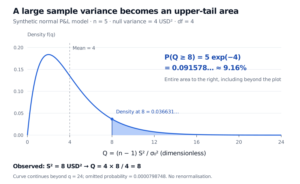
Original analytical plot for the synthetic example. The shaded probability includes the small tail beyond the displayed range; the plotted density is not renormalised. Density height at the cutoff is not the tail probability.
If a 5% significance level was fixed in advance, this upper-sided hypothesis test does not reject the stated variance. That does not establish that the variance equals 4 USD-squared. The 9.16% is the chance, under the complete null model, of obtaining a sample variance at least this large in another five-observation sample. It is not the probability that the null variance is true, nor a posterior probability that the variance exceeds a threshold. A two-sided variance question needs a two-sided rule; the upper tail alone answers a different question. NIST describes these separate variance-test alternatives.
When the reference law changes
Normality supplies the exact finite-sample variance law. Heavy-tailed P&L, serial dependence, changing conditional volatility or selection of the window after seeing its results can invalidate this calculation. Merely retaining the divisor does not restore it. The chi-squared family also appears as an asymptotic reference for other statistics, including goodness-of-fit tests; those have their own assumptions and degree counts.
The squared-normal construction above is central: the normal coordinates have mean zero and variance one. Squaring shifted normal coordinates generally produces a noncentral chi-squared law, while correlated or differently scaled coordinates need further analysis. “Sum of squares” alone does not identify a distribution.
For the derivation of the variance law and the loss of one degree of freedom, read The Sampling Distribution of S-squared and Cochran's Theorem, especially Theorem 2. The full lesson requires membership, with a public preview available. The same variance pivot can be inverted to form a confidence interval for population variance under the stated normal model.
Sources
- John A. Rice, Mathematical Statistics and Data Analysis, 3rd ed., §§6.2–6.3, especially Theorem B in §6.3 — squared-normal construction, moments, and the exact normal-sample variance distribution.
- NIST/SEMATECH e-Handbook: Chi-Square Distribution — density, support and shape properties.
- NIST/SEMATECH e-Handbook: Chi-Square Test for the Variance — variance statistic and one-sided versus two-sided alternatives.