The Gamma distribution models positive quantities and sums of exponential waits. Distinguish shape, rate and scale using the time to a third market event.
Gamma distribution
The Gamma distribution is a family of continuous probability distributions for positive quantities, controlled by a shape parameter and a scale parameter. It can describe the time until several events have occurred, or uncertainty about a positive quantity such as an event intensity. The same family serves these different roles; the meaning and units of the random variable must come from the model.
For an execution researcher, the distinction between the next event and the third event matters. Under a homogeneous Poisson process, the next-event wait is exponential; the third-event wait is Gamma. Neither clock, by itself, tells a trader when an order will fill.
and is zero for negative x. The normalising function is Γ(α)=∫0∞uα−1e−udu; for a positive integer n, Γ(n)=(n−1)!. The Gamma function is a mathematical function; the Gamma distribution is a probability law built using it.
Many books instead write shape–rate, with β=1/θ:
fX(x)=Γ(α)βαxα−1e−βx.
If X is measured in minutes, scale is measured in minutes and rate in inverse minutes; shape is dimensionless. “Gamma(3, 2)” is therefore incomplete documentation unless the second parameter's convention is stated. A scale of two minutes and a rate of two per minute describe very different waits.
These moments exist for every positive shape and scale. Scale stretches the horizontal axis. Shape changes relative dispersion as well as the curve's form.
A clock for the third market event
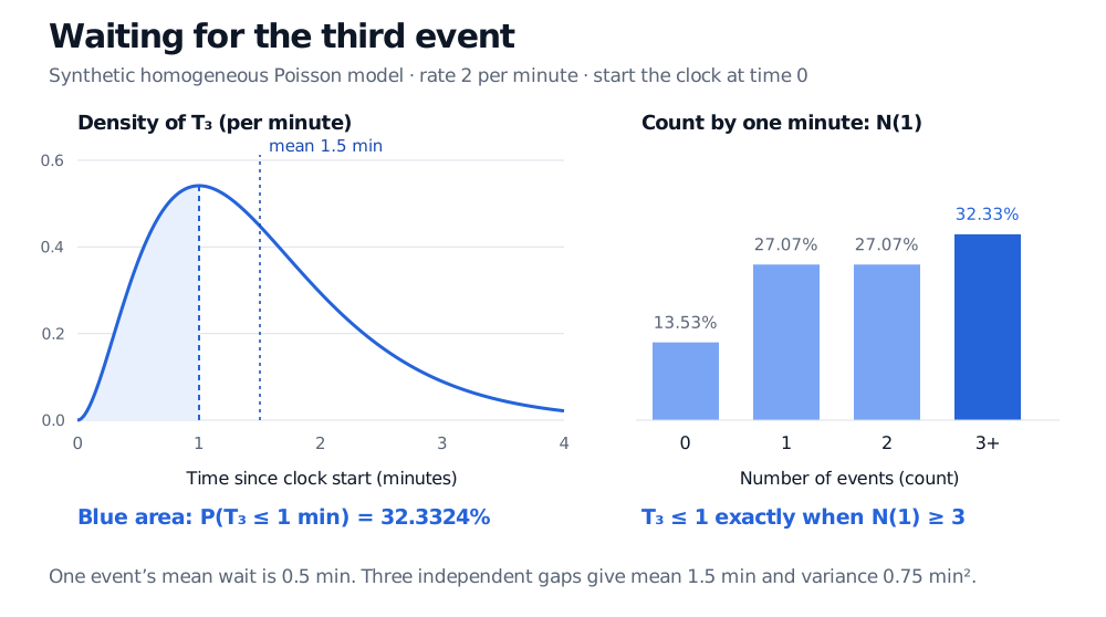
Suppose a researcher stipulates that qualifying quote updates follow a homogeneous Poisson process at two events per minute. Start the clock at time zero and let T3 be the time until the third update. Independent exponential gaps, each with rate two per minute, give
T3=τ1+τ2+τ3∼Gamma(shape 3, scale 0.5 min).
The equivalent shape–rate specification has rate 2 min−1. Consequently,
E[T3]=1.5 min,Var(T3)=0.75 min2.
The expected time is not a deadline. To ask whether all three updates arrive within one minute, change from the clock to the event count: T3≤1 exactly when N(1)≥3. Since N(1) has a Poisson distribution with mean two,
So the model assigns a 32.3324% chance to receiving the third update within one minute. The density at one minute is not this probability: probability is an area, or equivalently a count-tail event.
Gamma third-arrival density and equivalent Poisson count tail, with mean 1.5 minutes, variance 0.75 square minutes and 32.3324 percent probability of three or more events by one minute.Original stipulated arrival model: the shaded waiting-time area equals the final count bar. The density axis uses inverse minutes; the count bars show probabilities.
This is a synthetic arrival assumption, not an estimate of current market activity. Clustering, time-of-day changes and dependence between updates can invalidate the constant-rate model. Counting quote updates also supplies no queue position, trade direction or order-size information needed for a fill model.
Integer shape is a mechanism; noninteger shape is allowed
The sum of n independent exponential waits with a common rate is Gamma with shape n. This integer-shape case is also called an Erlang distribution. More generally, independent Gamma variables with a common scale add by adding their shapes. Arbitrary unequal scales do not have that closure property.
The family also permits α=0.5, 2.7 or any other positive real value. A noninteger shape is valid, but it does not literally mean waiting for “2.7 arrivals” in an ordinary counting process.
At α=1, Gamma reduces to the exponential distribution.
For α>1, the density rises from zero to an interior mode at (α−1)θ, then falls.
For 0<α<1, the density decreases from an infinite limit as x↓0. That integrable spike is not a positive probability of zero: P(X=0)=0 throughout the family.
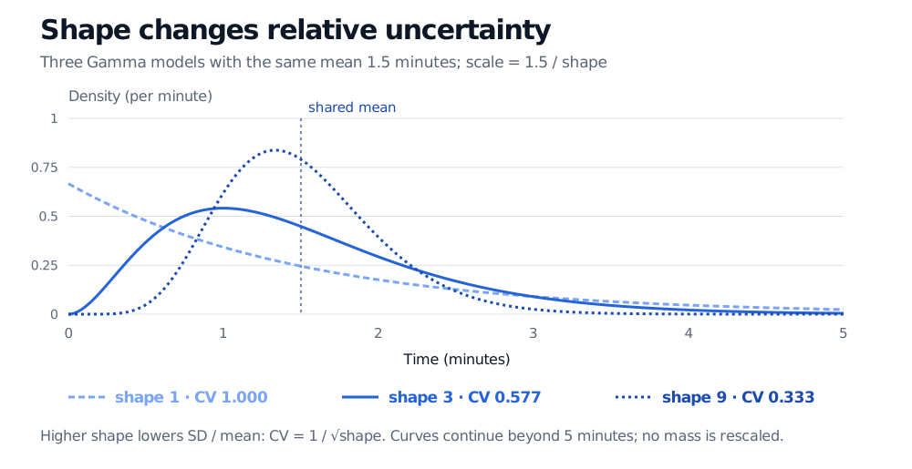
At a fixed mean, larger shape gives smaller relative uncertainty. In the next figure, all three means are 1.5 minutes, but the shape-nine model concentrates more tightly than the exponential shape-one model.
Gamma densities with shapes 1, 3 and 9 and a shared mean of 1.5 minutes. Their standard deviations divided by mean are respectively 1, 0.577 and 0.333; larger shape concentrates the distribution.Original model comparison. Scale is adjusted to 1.5 divided by shape in minutes. The finite plotting window does not truncate or renormalise the distributions.
A further special case is the chi-squared distribution: χν2 is Gamma with shape ν/2 and scale two. The corresponding rate is one-half.
Do not give every Gamma variable an exponential clock's memory
Only shape one is memoryless. In the third-arrival example,
P(T3>2∣T3>1)=5e−213e−4≈0.351872,
whereas P(T3>1)=5e−2≈0.676676. Knowing only that the third event has not arrived after one minute changes the remaining-wait distribution. If the full event history instead tells you exactly two events have occurred, the remaining wait is one fresh exponential gap; that is a different conditioning statement.
For noninteger shapes, probabilities normally use the incomplete gamma function, and quantiles generally require numerical inversion. Use a library's survival function for small upper-tail probabilities rather than subtracting a rounded cumulative probability from one.
Gamma is also useful as a prior distribution for a positive Poisson intensity. In that application, the random variable is the intensity itself, not a waiting time; its units and its Gamma parameters' units change accordingly. The conjugate-prior lesson develops that updating calculation. For the waiting-time construction, continue with sums of exponentials. Both full lessons require membership and have public previews.
Sources
Joseph K. Blitzstein and Jessica Hwang, Introduction to Probability, second edition (CRC Press, 2019), §8.4: Gamma density, moments, exponential sums and arrival times.