Prior probability is the starting probability before a specified observation. See how the same credit alert updates different priors, and how to avoid counting evidence twice.
Prior probability
A prior probability is the probability assigned to an event or hypothesis before incorporating a specified new observation. It describes the starting information for that update. After incorporating the observation, the updated probability is the posterior probability.
“Before” is relative to this observation, not to all data ever collected. A credit analyst's prior can already reflect earlier defaults, current balance sheets and a sector assessment. What matters is identifying which information is already included and which information the next update adds.
The useful prerequisite is conditional probability: probabilities depend on the information being conditioned on. If I denotes the starting information and E the new evidence, the distinction is
prior for this updateP(H∣I)⟶posterior after new evidenceP(H∣I,E).
Writing the prior simply as P(H) usually leaves that background information implicit.
One alert, two starting points
A credit desk monitors whether an issuer will default within the next year. Let H mean default within that horizon and E mean a new warning flag. Consider a hypothetical model, with all probabilities conditional on the same starting information:
The prior default probability is 5%.
The flag appears for 80% of issuers that default: P(E∣H)=0.80.
It also appears for 20% of issuers that do not default: P(E∣Hc)=0.20.
Here Hc is the complementary event, no default within the stated year. The numbers are model inputs, not estimated issuer forecasts.
The alert is four times as likely under default as under no default. That describes its relative evidential strength; it does not make the chance of default 80%. Bayes' theorem combines the flag's likelihood with the starting probability:
The 0.23 denominator includes both ways to produce an alert. In an illustrative population of 1,000 issuers with exactly the stipulated proportions, 50 default and 950 do not; 40 of the defaulting group and 190 of the non-defaulting group alert. Defaulting issuers are therefore 40 of the 230 alerted cases. These are implied model counts, not observed records.
Now change only the prior to 20%, keeping both conditional alert rates fixed:
P(H∣E)=0.80(0.20)+0.20(0.80)0.80(0.20)=50%.
Per 1,000 model issuers, 160 defaulting and 160 non-defaulting issuers now alert. The evidence mechanism is identical, but the composition of the population entering it has changed.
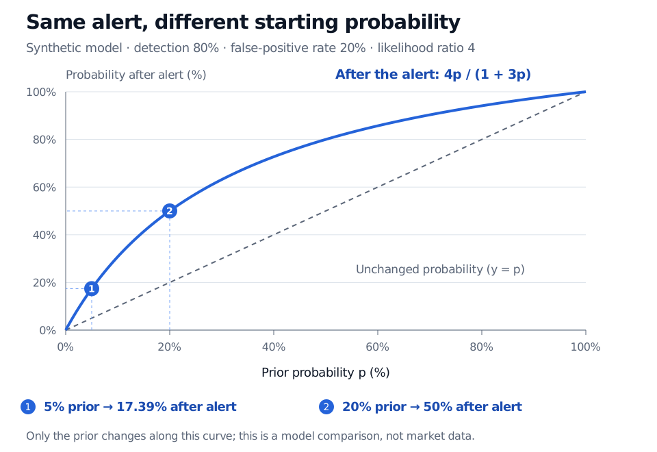
With alert detection 80% and false-positive rate 20%, a 5% prior becomes a 17.39% posterior and a 20% prior becomes 50%. The synthetic posterior-versus-prior curve lies above the unchanged-probability diagonal.
Original synthetic sensitivity comparison. The curve holds both conditional alert rates fixed; the filled points mark the two worked cases. Axes measure probabilities, not forecast accuracy.
For any prior p in this model, the posterior is 4p/(1+3p). The comparison reveals why a prior deserves scrutiny: the same evidence can support different final probabilities when the starting information differs. In actual credit populations, changing the issuer group may also change the conditional alert rates; holding them fixed is an explicit assumption here.
The odds form isolates the two contributions particularly clearly:
Odds of 4:19 correspond to probability 4/(4+19)=4/23. A factor of four multiplies the odds, not the 5% probability.
What justifies the starting probability?
A prior can come from a relevant historical population, a previous model update, structured expert judgement, or a combination with explicit assumptions. A historical default frequency is useful only after asking whether its horizon, issuer selection and economic conditions match the present question. A desk view should expose those choices rather than hide them inside a single number.
Two hypotheses do not automatically deserve probabilities of one half each. Equal weights express a specific judgement; the existence of two labels provides no evidence that the labels are equally likely. Likewise, a prior probability is not certainty. In a finite hypothesis model, assigning zero prior probability excludes that hypothesis from any defined ordinary Bayesian update, so a zero should represent a deliberate exclusion rather than casual disbelief.
For an uncertain numerical parameter, the corresponding object is a prior distribution over possible parameter values. Its mean alone does not describe how concentrated it is. Two priors can share a mean default rate while giving different weight to extreme rates and responding differently to a small new sample. This differs from the example above, where the prior is one probability for a fixed issuer-level event.
Keep an information ledger
A useful discipline is to write down “already included” and “newly observed” before updating. Yesterday's posterior can be today's prior when today's evidence is additional information. If the prior already incorporated a warning flag, multiplying by that same flag's likelihood again counts it twice.
For a genuinely new observation, use likelihoods conditional on the information already included. Reusing an unconditional detection rate after a previous alert requires justification; dependence between observations can change that rate. A well-documented prior and a poorly specified likelihood still produce a poorly specified posterior.
To practise separating these inputs, the SelfMadeQuant Bayes' rule trainer supplies prepared scenarios and asks you to estimate the updated probability. Guests can reveal one answer; continuing requires a free signed-in account. The examples in this article stand on their own; the trainer uses its own scenarios.
For the underlying probability rules, Probability Fundamentals is available in full with a free signed-in account. To study prior distributions and their strength, Bayesian Reasoning works through beta–binomial default-rate and normal–normal mean-return updates. Its full lesson requires membership; the public link provides a preview.
Sources
Bertsekas, D. P., and Tsitsiklis, J. N. (2008), Introduction to Probability, 2nd ed., §1.4 (Bayes' rule), Chapter 8 introduction and §8.1 (prior information and Bayesian inference).