Likelihood holds observed data fixed and compares model parameters. Distinguish sequence and count likelihoods, density and probability, log-likelihood and posterior probability.
Likelihood
Likelihood is the probability mass or density of the observed data, viewed as a function of a model’s unknown parameter. Hold the observations fixed and vary the parameter: which values assign the data greater mass or density?
If a model has joint mass or density fθ(x) and the observed sample is x, its likelihood is
L(θ;x)=fθ(x).
The formula is unchanged; the question has changed. A sampling distribution varies possible data at a fixed parameter. A likelihood varies candidate parameters at the data actually observed. Casella and Berger formalise this distinction in §6.3.1; Watkins’ university notes introduce it through Bernoulli and normal samples.
Seven profitable trades: what exactly was observed?
Consider a synthetic record of ten trades. Record 1 for a positive realised profit after costs and 0 otherwise:
x=(1,1,0,1,1,0,1,0,1,1).
For this illustration, stipulate independentBernoulli observations with one constant, unknown success probability p∈[0,1]. There are seven successes and three failures. For the particular ordered sequence,
L(p;x)=i=1∏10pxi(1−p)1−xi=p7(1−p)3.
Each success contributes p; each failure contributes 1−p. Independence justifies multiplication of the marginal masses, and the common p justifies combining the exponents.
Now suppose the recorded observation is only the total K=7. Under this model, K has a binomial distribution. There are (710)=120 different ordered sequences with seven successes, all equally probable at any fixed p. Therefore
Lcount(p;7)=120p7(1−p)3.
Candidate p
Particular ordered sequence
Count K=7
0.5
0.0009765625
0.1171875
0.7
0.0022235661
0.266827932
These columns concern different events. The count includes the observed sequence and 119 other possible arrangements. Its larger probability is not stronger evidence from extra observations. Penn State’s Bernoulli/binomial treatment explains this parameter-independent factor.
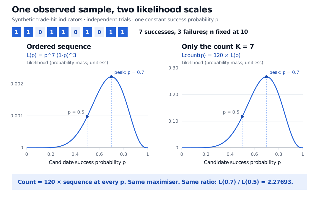
Two likelihood curves for ten independent Bernoulli observations with seven successes. The ordered-sequence curve peaks at p 0.7 with likelihood 0.0022235661. The count curve is 120 times larger and peaks at 0.266827932. Each gives likelihood ratio 2.27693 when comparing p 0.7 with p 0.5.
Original synthetic example. The vertical scales differ: multiplying by 120 changes the height, while preserving the peak and every within-column likelihood ratio.
For either representation, the likelihood ratio comparing p=0.7 with p=0.5 is
L(0.5;x)L(0.7;x)=2.2769316864.
Thus the observed data receive about 2.277 times as much probability mass under the first candidate. This is neither the probability that p=0.7 is true nor a probability that the strategy will be profitable in future. Win frequency also omits win and loss magnitudes: it cannot establish positive expected profit.
Products become sums, avoiding underflow from multiplying many tiny masses or densities. Because logarithm is strictly increasing, it preserves the maximiser and comparisons. Here
ℓ′(p)=p7−1−p3,ℓ′′(p)=−p27−(1−p)23<0.
The unique interior maximum is p^=7/10=0.7, the maximum likelihood estimate. Both endpoints have likelihood zero because the sample contains successes and failures; their log-likelihood is −∞. The count log-likelihood adds only log120, so it has the same maximum. This is an estimate under the stipulated model, with substantial sampling uncertainty from just ten observations.
Continuous observations use density
If a return has an ordinary probability density, its probability of equalling any one exact value is zero. Nevertheless its density at an observed value can be positive, and that density supplies the likelihood. For a short interval where the density is continuous,
Pθ(x≤X≤x+h)≈fθ(x)h.
The interval width turns density into approximate probability; it is not part of the density itself. MIT’s maximum-likelihood reading develops this small-interval interpretation.
For example, model one decimal return as normal with mean 0.005 and standard deviation 0.01. At an observed return of 0.005, the density is approximately 39.8942 per unit of decimal return. A density above one is valid. Express the same observation in percentage points instead: the observation and mean are 0.5, the standard deviation is 1, and the density is 0.398942 per percentage point. The economic observation has not changed; the density’s units have.
This is why raw likelihood heights need context. Compare candidate parameters using the same observations, model and data representation. A parameter-independent scaling cancels from ratios, as with the count factor or this unit conversion. Changing the sample, observation rule or parameter-dependent parts of the model requires rebuilding the likelihood; do not compare unrelated printed heights.
Assumptions travel with the likelihood
Likelihood itself does not require independence: the general definition uses the joint mass or density. With dependent trades, it may instead factor into an initial distribution and successive conditional distributions. Overlapping positions, common market shocks and changing regimes can invalidate the simple Bernoulli product. Even with independence, unequal success probabilities would require separate factors rather than a single common p.
Finally, likelihood alone is not a posterior distribution over the parameter. Bayesian inference combines it with a prior and normalises the result. Merely reading a likelihood height as “the probability of this parameter” reverses the conditioning without supplying that additional model.
For a fuller derivation, Estimation and Maximum Likelihood develops Bernoulli and normal estimators, boundary cases and model misspecification. A public preview is available; the complete lesson requires membership.
Sources
Casella, G. and Berger, R. L., Statistical Inference, 2nd ed., §6.3.1, “The Likelihood Function.”