Log-likelihood turns data likelihood products into sums without changing the best fit. Compare fill-probability candidates, distinguish sequence from count data, and handle boundaries and density units.
Log-likelihood
The log-likelihood is the natural logarithm of a likelihood, viewed as a function of a model's parameters with the observed data held fixed. It ranks candidate parameters exactly as the likelihood does, while replacing products by sums. This makes it the working objective for fitting fill probabilities, default models and return distributions.
Write x=(x1,…,xn) for the observations and θ for the unknown parameter or parameter vector. If the observations are independent and identically distributed with probability mass or density f(xi;θ), then
Throughout this page, log means the natural logarithm. Because it is strictly increasing on positive numbers, maximising ℓ gives the same parameter estimates as maximising L. At a zero likelihood, use the extended value ℓ=−∞. Neither function is a probability distribution over θ: the data are fixed while the parameter varies. UC Berkeley's maximum-likelihood notes derive this distinction and the Bernoulli case.
Seven fills, three misses
Suppose a desk records whether each of ten comparable limit orders fills within a fixed observation window. A fill is 1 and a miss is 0. Consider this synthetic ordered sample:
x=(1,0,1,1,0,1,1,1,0,1).
Assume an IID Bernoulli model with a common fill probability p∈[0,1]. This is a deliberate simplification: order size, queue position and market conditions are held outside the example. Seven fills and three misses give
L(p;x)=p7(1−p)3,ℓ(p;x)=7logp+3log(1−p),0<p<1.
Each observed fill contributes logp; each miss contributes log(1−p). Increasing p helps explain the fills but makes the three misses harder to explain. The optimum balances both contributions.
Candidate p
Ordered-sample likelihood L(p;x)
Natural log-likelihood ℓ(p;x)
0.5
0.0009765625
−6.931472
0.7
0.0022235661
−6.108643
0.9
0.0004782969
−7.645279
The largest entry in each objective column occurs at 0.7. A less negative log-likelihood is larger. The value −6.108643 is not a negative probability, and p=0.7 does not mean there is a 70% probability that the parameter estimate is correct.
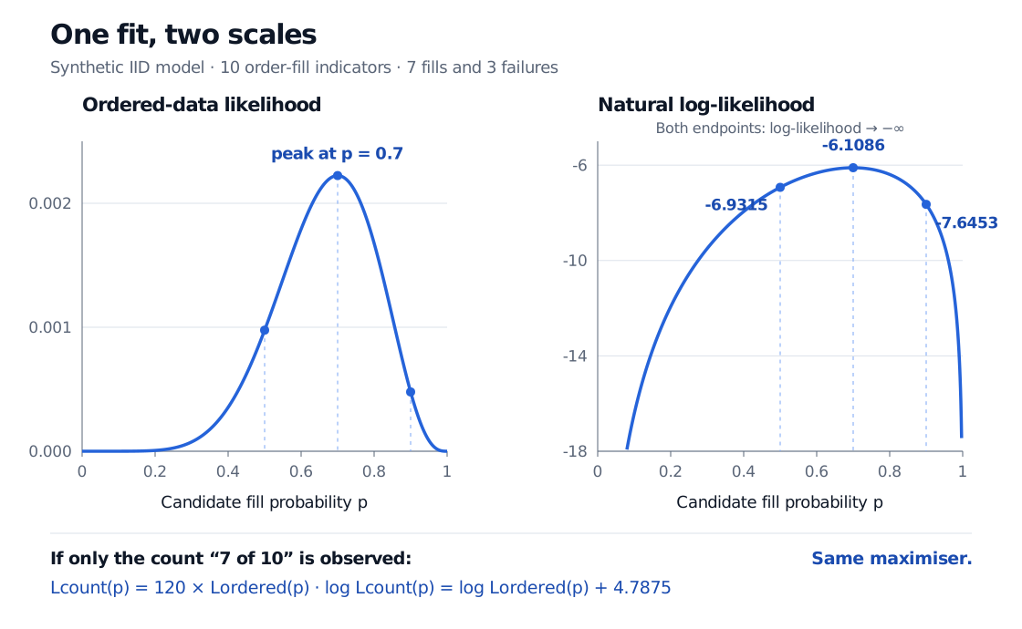
For ten synthetic IID fill indicators with seven fills, ordered likelihood and natural log-likelihood both peak at candidate fill probability 0.7. Log-likelihoods at 0.5, 0.7 and 0.9 are −6.9315, −6.1086 and −7.6453. The binomial count log-likelihood is shifted upward by log 120, or 4.7875.
Original synthetic Bernoulli example. The horizontal axes vary the candidate parameter, with the observed sample fixed. The right panel omits the unbounded tails: both endpoint log-likelihoods are −∞.
For an analytic check, differentiate in the interior. The score function and second derivative are
ℓ′(p)=p7−1−p3,ℓ′′(p)=−p27−(1−p)23<0.
The score vanishes when 7(1−p)=3p, giving the maximum likelihood estimatep^=7/10=0.7. Strict concavity makes this the unique maximum; at p=0 the observed fills are impossible, and at p=1 the observed misses are impossible. Both boundaries have likelihood zero.
Did you observe an ordered sequence or a count?
If the recorded observation is only “seven fills out of ten,” its binomial probability mass includes every ordering with seven fills. There are (710)=120 such sequences, so
Lcount(p)=120p7(1−p)3,ℓcount(p)=log120+ℓ(p;x).
At p=0.7, the count probability is 0.266827932, whereas the probability of the particular ordered sequence is 0.0022235661. These describe different observed events. The factor 120 does not depend on p, so it changes the absolute log-likelihood by 4.787491743, but changes neither the maximiser nor a likelihood ratio between candidate values of p.
You may omit such constants to find an optimum. Keep track of what was omitted when reporting a log-likelihood or comparing software results; two absolute values with different conventions need not agree. A relative profile exp{ℓ(p)−ℓ(p^)} peaks at 1, but still does not sum or integrate to 1 as a distribution over p.
What taking logs fixes—and what it cannot fix
It avoids multiplying tiny numbers. With 7,000 fills and 3,000 misses under the same IID model, the ordered log-likelihood at p=0.7 is approximately −6108.643021. The corresponding product underflows to zero in ordinary double-precision arithmetic. Evaluate the log terms directly; taking a log after the product has already rounded to zero loses the information. Near p=0, software's log1p(-p) evaluates log(1−p) without first subtracting two nearly equal numbers.
It does not remove boundaries. For an all-fill sample, L(p)=pn is maximised at p=1 if that value is allowed. An all-miss sample is maximised at p=0. Evaluate these cases directly or by limits, using 0log0=0 for a zero-count contribution. Do not evaluate an undefined product of zero and an infinite log in software. If the parameter space is strictly (0,1), these samples have a supremum at an excluded boundary and no attained MLE. Replacing p by a small positive floor changes the objective and must not be presented as the exact likelihood.
It does not make every log-likelihood negative. A continuous probability density can exceed 1. For example, a uniform waiting-time model on (0,0.1) seconds has density 10 per second throughout that interval. An interior observation has log-density log10>0, although its exact-point probability is zero. Express the same time in milliseconds and the density is 0.01 per millisecond: the log-density changes by −log1000. Absolute continuous-data log-likelihoods depend on units and the density convention. Compare models using the same observations, units and reference measure; a larger raw number from a different scale is not evidence of a better fit.
It does not create independence. For dependent observations, the joint log-likelihood can instead be factored into conditional contributions:
ℓ(θ;x)=logfθ(x1)+i=2∑nlogfθ(xi∣x1,…,xi−1).
Logs still turn the product into a sum; the terms now describe conditional laws. Dropping history and multiplying marginal fill probabilities would impose a different model. Cosma Shalizi's Carnegie Mellon notes show this construction for Markov chains. A good numerical optimum cannot establish that IID fills, a chosen return distribution or a stable market regime is an adequate description of the data.
For further worked Bernoulli and normal-return fits, including boundary cases and the conditions behind information-based standard errors, see Estimation and Maximum Likelihood. The public preview gives the outline; the full lesson requires membership.
Sources
Larry Wasserman, All of Statistics: A Concise Course in Statistical Inference, Springer, §9.3, Definitions 9.7–9.8, Remark 9.9 and Example 9.10: likelihood, log-likelihood, parameter-independent factors and Bernoulli estimation.
John A. Rice, Mathematical Statistics and Data Analysis, 3rd edition, §8.5: joint likelihood, natural logarithms and IID factorisation.