Maximum likelihood estimation fits model parameters by maximising the data likelihood. Derive an exponential arrival rate, check the maximum, and distinguish best fit from uncertainty and truth.
Maximum likelihood estimation
Maximum likelihood estimation (MLE) estimates an unknown parameter by choosing a permitted value that maximises the observed data's joint probability mass or density under a specified model. It supplies a fitting rule for models of returns, defaults and event arrivals. The result is an estimate supported by that model and sample, with uncertainty attached.
Start with a likelihoodL(θ;x): hold the observed data x fixed and vary the candidate parameter θ over its domain Θ. An MLE satisfies
θ^∈θ∈ΘargmaxL(θ;x).
The set notation allows more than one maximiser. Some problems have none. The domain matters: a rate must be positive, a probability must lie in its allowed interval, and a covariance matrix must satisfy the model's matrix restrictions. TU Delft's introduction illustrates the change of viewpoint from density as a function of observations to likelihood as a function of parameters.
For continuous observations, an exact sample has probability zero. MLE compares densities; it does not maximise the probability of observing precisely those real numbers. Nor does L(θ;x) generally integrate to one over θ. A maximising parameter is not automatically the true parameter or a posterior probability. Bayesian inference requires a prior and normalisation of prior times likelihood.
An arrival-rate estimate, from assumptions to answer
Suppose an analyst records three synthetic waiting times between successive trades: 2, 3 and 5 seconds. To keep the fitting problem transparent, assume these are three complete, accurately measured observations from independent, identically distributed exponential waiting times, with one constant rate λ>0 per second:
f(t;λ)=λe−λt,t≥0.
This model says arrivals have a constant rate and memoryless waits. Real trade arrivals can cluster, change through the day and depend on market state. The assumption is a teaching model, not a statement that an exchange queue follows this law. Also assume the observation plan obtains three complete waits: no unfinished final interval, censoring, missing trades or selective removal of long waits. Those observation mechanisms can change the likelihood.
Independence makes the joint density a product. With n complete waits,
L(λ;t)=i=1∏nλe−λti=λne−λ∑iti.
A dependent model needs its joint or conditional densities instead; multiplying marginal densities would impose an assumption the data may not support.
It is easier to maximise the log-likelihood. The logarithm is strictly increasing, so it preserves the maximiser while turning products into sums. For these waits, whose total is 10 seconds,
ℓ(λ)=3logλ−10λ.
Here times are entered numerically in seconds and rates in inverse seconds. Changing the time unit changes the numerical rate and adds a parameter-independent constant to the corresponding log-density; the fitted physical rate is unchanged.
The score is the first derivative; curvature comes from the second:
ℓ′(λ)=λ3−10,ℓ′′(λ)=−λ23<0.
Setting the score to zero gives
λ^=103=0.3 per second.
This is a global maximum: the log-likelihood is strictly concave on the entire domain λ>0, and tends to −∞ as λ approaches zero or grows without bound. The fitted mean waiting time is 1/λ^=10/3≈3.3333 seconds. In general, the rate MLE is n/∑iti, the reciprocal of the sample mean. Taboga derives the exponential-model likelihood and its information.
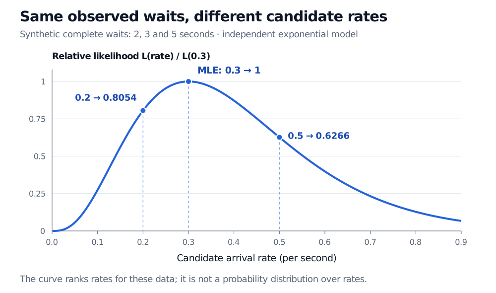
For synthetic complete waits of 2, 3 and 5 seconds, the relative likelihood peaks at rate 0.3 per second with value 1. At candidate rates 0.2 and 0.5 per second it is 0.8054 and 0.6266. The horizontal axis is candidate rate, not waiting time.
Original synthetic exponential-model example. Dividing by the maximum makes the peak one; it does not turn the curve into a probability distribution over rates.
For example, the log-likelihood is approximately −6.6119 at 0.3 and −6.8283 at 0.2. Thus the latter candidate has relative likelihood L(0.2)/L(0.3)≈0.8054. That is a comparison of support within this model, not an 80.54% probability that the rate equals 0.2.
A best fit still needs an uncertainty assessment
Before sampling, an estimator is a function of random observations. After sampling, 0.3 is its realised estimate. A fresh set of three waits would generally give another value.
Curvature measures how sharply the likelihood falls near an interior maximum. For one scalar parameter, the observed information is J(θ^)=−ℓ′′(θ^). Under suitable large-sample regularity conditions, its inverse square root estimates a standard error. In the exponential example,
J(λ^)=0.323=33.3333… seconds2,SE(λ^)=3λ^≈0.1732 per second.
Three observations are too few to trust a normal approximation merely because this formula exists. This is a large-sample plug-in calculation, not an exact finite-sample uncertainty statement. Exact sampling methods for this exponential model, or a carefully justified likelihood-based interval, can provide a more appropriate confidence interval.
MLE also need not be unbiased. Under this same iid exponential model, for n>1 its exact expectation is E[λ^]=nλ/(n−1). With three waits that is 1.5λ, so the rate estimator has upward bias even though it genuinely maximises the likelihood. An observed estimate of 0.3 does not imply that the unknown rate is either 0.3 or 0.2.
The usual consistency and information-based uncertainty results require conditions including an identifiable, correctly specified model, adequate smoothness and control of the maximisation problem. They are not consequences of finding a score root alone. At boundaries, or with several local maxima, checking only a zero derivative can miss the answer.
What to check on financial data
A converged numerical optimiser establishes little about model risk. Check the observation mechanism, parameter restrictions, dependence, changing regimes and distributional fit. A constant exponential rate fitted to clustered trade arrivals may summarise their average pace while missing the very bursts that matter for execution risk. Under misspecification, the likelihood can still have a well-defined maximiser; standard model-based errors and forecasts may nevertheless be wrong. Suitable robust uncertainty methods address some estimation problems but cannot make an unsuitable model describe the market.
For fuller worked Bernoulli-default and normal-return derivations, along with boundary cases and information-based errors, see Estimation and Maximum Likelihood. A public preview is available; the full lesson requires membership.
Sources
Larry Wasserman, All of Statistics: A Concise Course in Statistical Inference, Springer, §§9.3–9.7: likelihood, maximisation, equivariance, consistency and information-based uncertainty.