Posterior probability is a hypothesis probability after observing evidence. A risk-alert example separates it from detection rate and evidence probability.
Posterior probability
Posterior probability is the probability assigned to a hypothesis after conditioning on observed evidence, under a specified probability model and the information already available. It answers “given what we have seen, how probable is this hypothesis?” A risk monitor's detection rate answers a different question: how often it alerts when stress occurs.
Here the conditional evidence rate P(E∣H) also requires P(H)>0 in this elementary event formulation. The prior probabilityP(H) describes the hypothesis before this observation; it can already incorporate earlier data. “Posterior” and “prior” name roles relative to an update, rather than two permanent kinds of probability.
A strong detector can leave stress unlikely
Suppose a desk defines H as an index losing at least 3% from today's open to close. An alert E is observed at the open. Use these hypothetical model inputs, not estimates of a real monitor:
Prior chance of the defined stress event: 2%.
Alert rate on stressed days: 90%.
Alert rate on non-stressed days: 10%.
Non-stress includes smaller losses as well as gains. The alert arrives before the closing outcome; no closing information is used to form the morning estimate.
An illustrative population of 10,000 model days makes the denominators visible:
Closing outcome
Alert at open
No alert
Total
Stress
180
20
200
Non-stress
980
8,820
9,800
Total
1,160
8,840
10,000
These are expected counts implied by the assumptions, not a reported backtest. Once an alert is observed, keep the 1,160 alerted cases. The 180 stressed cases within this group give
P(H∣E)=1160180=589≈15.52%.
The alert raises the stress probability substantially from 2%. Nevertheless, stress remains less probable than non-stress among alerted days: the much larger non-stress population contributes 980 false alerts. A 90% detection rate is not a 90% posterior.
This 11.6% is the chance that an alert appears before we observe it. It is neither the 90% likelihood under stress nor the 15.52% posterior stress probability after an alert. Observing an alert selects that part of the population; it does not make the stress hypothesis certain.
No alert is also information
If the monitor stays quiet, use the other column. Only 20 of the 8,840 non-alerted cases are stressed:
P(H∣Ec)=884020=4421≈0.226%.
The complementary eventEc means “no alert,” not “no stress.” The monitor misses some stressed days, so a quiet screen lowers risk without eliminating it.
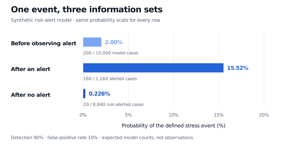
Stress probability is 2% before observing the alert, 15.52% after an alert and 0.226% after no alert. All three horizontal bars share a zero to twenty percent scale. Their denominators are respectively 10,000 model days, 1,160 alerted days and 8,840 non-alerted days.
Original synthetic model. Each bar measures the same stress event with a different information set. Counts are expected model counts, and all bars use the same probability scale.
The two posteriors also fit together. Before seeing the screen, weighting each by the probability of its observation recovers the prior:
0.116(589)+0.884(4421)=0.02.
An alert and no alert are alternative observations for the same day. They are not two successive updates to apply together.
What the number does and does not establish
The posterior is conditional on the model, event definition and available information. A different base rate or a monitor whose detection rates change across regimes gives a different result. Calculation alone does not establish that the inputs are well estimated or that the forecast is calibrated.
Nor does a posterior establish causation: an alert may be associated with stress without causing it. It also does not choose a trade. Position size requires the consequences of stress, possible gains, hedge costs and the decision-maker's objectives as well as a probability.
If further evidence arrives, the current posterior can become the next prior. The next likelihood must describe that evidence conditional on what has already been observed. Reusing the same alert, or treating correlated monitors as independent confirmations, can double-count information; multiplying separate likelihood ratios needs the relevant conditional independence assumptions.
For a continuously distributed parameter, a posterior density height is not a probability. Posterior probabilities of parameter ranges come from integrating the posterior density over those ranges. Likewise, exact continuous observations require density-based conditioning rather than inserting a zero-probability event into the elementary ratio above.
Put the interpretation to work
The SelfMadeQuant Bayes' rule trainer lets you estimate posteriors in prepared scenarios, then inspect the evidence-matching population. One answer reveal is available to guests; continuing requires a free signed-in account. Its scenarios practise the conditioning direction illustrated here.
For the step from a binary hypothesis to an uncertain default-rate or return parameter, Bayesian Reasoning develops beta–binomial and normal–normal posterior distributions. The public page previews the lesson; full access requires membership.
Sources
John A. Rice, Mathematical Statistics and Data Analysis, 3rd ed., §1.5, “Conditional Probability”: Bayes' rule, evidence and updated hypothesis probabilities.