Model risk arises when flawed, misestimated, incorrectly implemented or misused models distort decisions. A fixed-portfolio correlation example shows what sensitivity and validation can establish.
Model risk
Model risk is the possibility of adverse consequences from relying on a model that is wrong, poorly implemented, or used beyond what its evidence and assumptions support. A risk report can underestimate exposure; a pricing model can suggest a misleading hedge; a trading backtest can turn a chance pattern into a position.
The model is more than a formula. Its data, parameter estimates, software, reporting and the decision made from its output all matter. A mathematically correct calculation can still support a bad decision if it answers the wrong question.
Model risk is also different from an ordinary investment loss. A model that assigns a loss a positive probability has not necessarily failed when that loss occurs. Conversely, a profitable trade does not prove its supporting model was sound.
Four ways the chain can fail
These are useful diagnostic categories, rather than mutually exclusive boxes:
Source of risk
What can go wrong?
A useful challenge
Specification
The model leaves out a mechanism that matters for its intended use: jumps, changing dependence, transaction costs or funding constraints.
Compare a simpler benchmark and an alternative with meaningfully different assumptions. Which decisions change?
Estimation
The chosen structure may be reasonable, but its parameters are estimated imprecisely from noisy or unrepresentative data.
Perturb inputs, change defensible estimation windows, and examine uncertainty in the resulting decision.
Implementation
The intended model is translated incorrectly: a percentage is treated as a decimal, a covariance cross-term is omitted, or future information enters a backtest.
Reproduce small cases independently; check units, timing, boundary cases and the complete data-to-report chain.
Misuse
An output is applied to a different product, horizon or decision, or a conditional estimate is presented as a guarantee.
State intended uses, restrictions and what the output does not measure; examine how users actually act on it.
For example, assuming constant correlation is a specification choice; estimating that correlation from a short sample creates estimation uncertainty. Continuing to use the estimate after a major change in the assets can bring both problems together. More complex models can address a missing mechanism while introducing additional parameters and operational dependencies.
A correlation assumption changes the report
Suppose a hypothetical portfolio invests 50% in each of two assets, with no leverage. Both assets have 20% standard deviation of one-year simple total returns, measured in the same currency. These are stipulated inputs, not estimates from observed prices.
Here ρ is the assumed correlation, and σi is each asset's return standard deviation. Substituting the inputs gives
σp2=0.02(1+ρ).
Correlation assumption
Variance, decimal-return squared
Portfolio annual standard deviation
Baseline: 0
0.020
14.1421%
Alternative: 0.8
0.036
18.9737%
Estimated standard deviation rises by about 4.83 percentage points, or 34.16% relative to the baseline. The holdings have not changed. What changed is the reported risk under a different dependence assumption.
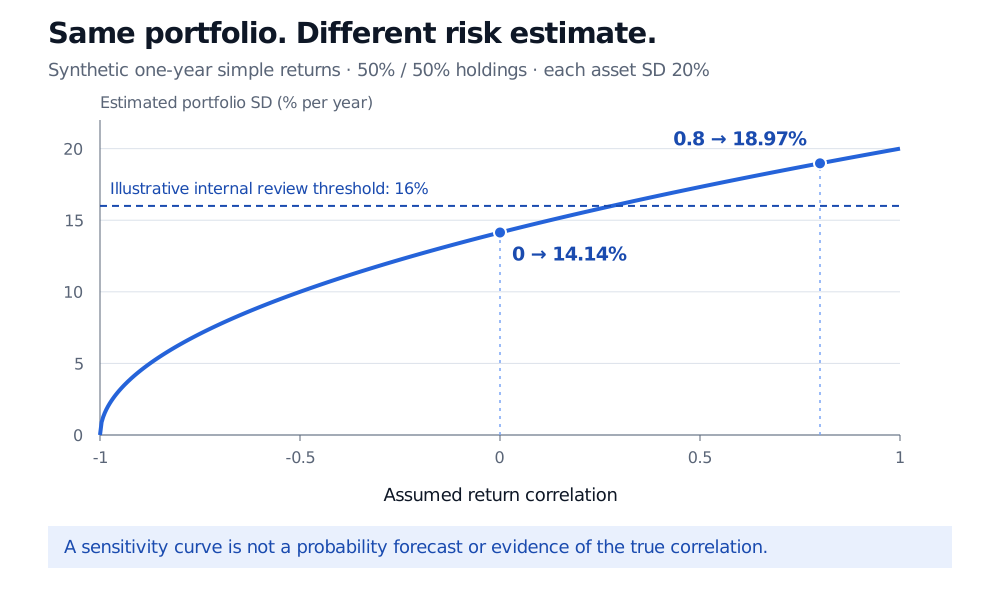
Imagine an internal review threshold of 16% annual standard deviation. The baseline report is below it; the alternative report is above it. Indeed, this model crosses that threshold at ρ=0.28. The threshold is an illustrative decision rule, not a regulatory limit.
With fixed 50 percent holdings and 20 percent annual standard deviation for each asset, assumed correlation 0 gives portfolio standard deviation 14.14 percent and correlation 0.8 gives 18.97 percent. An illustrative 16 percent internal review threshold is crossed at correlation 0.28.
Synthetic one-year simple-return sensitivity. The asset standard deviations and holdings stay fixed; only assumed correlation changes. The dashed line is an illustrative internal review threshold.
This is a sensitivity analysis: it shows that a decision is sensitive to a load-bearing input. It does not establish that 0.8 is the true correlation, give a probability that correlation will reach it, or show that 18.97% is the largest possible risk. Other inputs can change too. Even fixing all variances and correlations does not specify a full joint return distribution or its tail losses.
The formula provides useful implementation checks: correlation 1 gives 20% portfolio standard deviation; correlation −1 gives zero in this exact equal-volatility, equal-weight model. That zero follows from perfect offsetting return deviations under the stipulated model. It is not evidence that two real assets provide a riskless trade.
The Expectation, Variance and Covariance lesson develops the calculation and the distinction between zero covariance and independence. Full access requires a free signed-in account; the public page provides a preview.
Validation should challenge the decision
Model validation asks whether a model is sufficiently reliable for a specified use, and what limits remain. In the example, reproducing the variance calculation checks implementation. It does not validate the correlation input. A useful review would also ask why the estimation window represents the intended holding period, whether assets and currencies are aligned, and whether the decision remains acceptable under plausible alternatives.
Backtesting adds evidence from outcomes, but its strength depends on the observations available and how the test was designed. Repeatedly changing a model after seeing its test results can create overfitting. A quiet historical sample provides little direct evidence about an unobserved crisis. Two models agreeing is weak reassurance when both omit the same risk.
Pricing offers another useful challenge. Fitting today's vanilla option prices does not, by itself, determine the joint evolution of prices across future dates. A path-dependent contract can depend on features that vanilla calibration leaves unresolved. Hull discusses this in §27.3; Hull and Suo's study illustrates why model-risk conclusions depend on the product being priced and hedged. An alternative model is a challenger, not an oracle, and a two-model price range is not automatically a confidence interval or a worst-case bound.
Validation therefore supports a conditional judgment, not a certificate of truth. Useful controls connect findings to action: an accountable owner, documented assumptions, limits on use, monitoring triggers, and a response when performance or inputs deteriorate. Scrutiny should reflect the consequences of error as well as mathematical complexity. The 2026 interagency guidance makes both residual risk after validation and proportionate review explicit.
Regulatory references need context. The Federal Reserve's SR 26-2, issued 17 April 2026, superseded SR 11-7 and is most relevant to Federal Reserve-regulated banking organizations above USD 30 billion in assets. The agencies describe the guidance as principles rather than enforceable standards or prescriptive requirements. It is not a universal legal rule or a fixed validation calendar for every quant model.
Sources
Elton, E. J., Gruber, M. J., Brown, S. J. and Goetzmann, W. N. (2014). Modern Portfolio Theory and Investment Analysis, 9th edition, Chapter 4, pp. 51–53: two-asset variance, covariance and correlation.
Hull, J. C. (2018). Options, Futures, and Other Derivatives, 9th Global Edition, §§27.2–27.3: stochastic volatility, calibration and the limits of the implied volatility function model.