Parameter: Definition & Examples

A parameter is a quantity that specifies a model or selects a member of a family of functions or distributions. For a quant, it might be a return model's mean, a default probability or a regression coefficient. A parameter can be supplied as an assumption, estimated from data or calibrated to prices. Its role comes from the model, rather than from the letter used to name it.

For example, in the family

f(x;a)=ax

x

is the input and

a

controls the slope. Holding

a

fixed gives one function; changing

a

selects another. If the task is to fit the slope, that same

a

becomes the unknown quantity to infer. If the task is to choose a portfolio allocation, the quantity being chosen is instead a decision variable. The distinction depends on the problem.

A return is not its model's mean

Suppose a risk analyst specifies this deliberately simplified stationary model for one-day log returns, expressed as decimals:

R\sim\mathcal{N}(\mu,\sigma^2), \qquad \mu=0.001,\quad \sigma=0.02.

Here

\mathcal{N}

denotes the normal distribution. The random variable

R

represents a return before it is known. The parameters describe its probability distribution:

\mu

is the expected value, while

\sigma

is its standard deviation. In this notation the second argument is variance:

\sigma^2=0.02^2=0.0004.

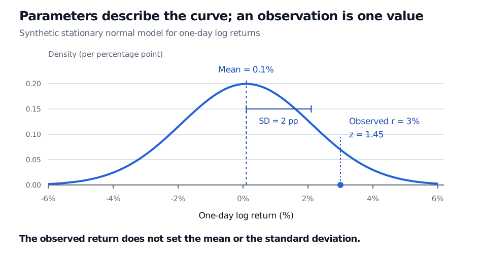
The horizon and units matter. This is a mean of 0.1% and a standard deviation of 2 percentage points for a one-day log return. Variance is in squared decimal-return units; in percentage-point coordinates it is $2^2=4$ squared percentage points. These are daily distribution inputs, not annualised drift or volatility inputs for a continuous-time model. We require $\sigma>0$ for the non-degenerate normal density used here.

Now the next day produces the observation $r=0.03$ , a 3% log return. Its standardised distance from the assumed mean is

z=\frac{r-\mu}{\sigma} =\frac{0.03-0.001}{0.02}=1.45.

The return lies 1.45 standard deviations above the model mean. It does not replace $\mu$ with 3%, and it does not reveal the true volatility. The score measures a distance, not the probability of that exact return. Under a continuous normal model, any single exact value has probability zero; probabilities come from intervals.

Synthetic normal daily log-return density with mean 0.1%, standard deviation 2 percentage points, and an observation at 3%, which is 1.45 standard deviations above the mean.

Original synthetic stationary normal model. The horizontal axis uses percentages and the vertical axis density per percentage point. Parameters specify the curve; one realised return supplies the marker.

Unknown parameter, estimator, estimate

In classical estimation, an unknown parameter is treated as fixed within the assumed model. The data vary across hypothetical repeated samples. That creates five different objects:

Object	In this example	Role
Parameter	$\mu$	Mean of the model distribution; possibly unknown
Random variable	$R_i$	A daily log return before observation
Observation	$r_i$	The recorded value of that return
Estimator	$\hat\mu=\frac{1}{n}\sum_{i=1}^{n}R_i$	Rule applied to random data; random before observing the sample
Realised estimate	$\hat\mu(r_1,\ldots,r_n)$	The numerical output after the data are supplied

For a separate synthetic historical sample of five log returns, $(-0.01,0,0.005,0.008,0.0035)$ , the sample mean is $0.0013$ , or 0.13%. That is one realised estimate of $\mu$ , not proof that $\mu=0.0013$ . Another sample generally gives another estimate. Five observations are used only to make the arithmetic visible, not to suggest adequate precision for estimating a financial mean.

An estimator therefore has sampling uncertainty even when the target parameter is fixed. Plugging its realised value into a model does not remove that uncertainty. The Estimation and Maximum Likelihood lesson develops this distinction and the normal mean/variance estimates. Its public page is a preview; the full lesson requires membership.

“Parameter” does not mean permanently constant

Constant parameters are an assumption of the stationary example above. Other models specify time-varying coefficients, conditional means or stochastic volatility. Bayesian inference represents uncertainty about unknown parameters with a prior and posterior distribution. None of these uses turns a model parameter into an observed return.

Nor does a plausible fitted parameter guarantee a suitable model. Returns may have heavier tails or changing volatility, so a precisely estimated normal model can still describe risk poorly. Keep separate uncertainty about the parameter and error in the model family. The Normal Distribution primer develops standardisation and this tail-risk limitation; the full lesson is available with a free signed-in account, with a public preview before sign-in.

In software, “parameter” can also mean a function argument, and “hyperparameter” often means a setting governing how a model is fitted. An argument may carry a model parameter, an observed price or a training setting. Check the mathematical role and units rather than assuming every input is the same kind of object.

Sources

Dimitri P. Bertsekas and John N. Tsitsiklis, Introduction to Probability, 2nd edition, Athena Scientific, 2008, §9.1, “Classical Parameter Estimation”; Chapter 8 provides the Bayesian contrast.
NIST/SEMATECH e-Handbook of Statistical Methods, §1.3.6.6.1: Normal Distribution, for normal parameters and their estimation.
NIST/SEMATECH e-Handbook of Statistical Methods, §1.3.6.4: Location and Scale Parameters, for how location and scale select a distribution. The return scenarios and diagram here are original.

A return is not its model's mean

Unknown parameter, estimator, estimate

“Parameter” does not mean permanently constant

Sources

Related terms

Decision variable

Estimator

Expected value

Normal distribution

Probability distribution

Random variable

Standard deviation