A decision variable is a quantity an optimisation problem chooses. Separate portfolio weights from model inputs and uncertain returns in a two-asset example.
Decision variable
A decision variable is a quantity whose value an optimisation problem asks us to choose. In portfolio construction, weights or trade sizes can be decision variables; future market returns cannot be selected by choosing a weight. Identifying the choices correctly is the first step in turning an investment question into a mathematical model.
A decision variable needs a meaning, units and a domain. A weight might be a continuous fraction of capital; a number of contracts might be an integer. The constraints restrict admissible choices, and the objective function scores them. Naming a symbol x does not tell us which role it plays.
One choice determines two weights
Consider a synthetic one-period allocation between fictional assets A and B. We choose the fraction w invested in A and put the remainder 1−w in B. The portfolio is fully invested and long-only, with a hypothetical 60% cap on A:
0≤w≤0.6,wB=1−w.
Here w is the one independent decision variable. We could instead write two variables, wA,wB, and impose wA+wB=1. These are equivalent descriptions of the same choices: two named weights do not give two independent degrees of freedom once the budget equation is imposed. The feasible set runs from all capital in B to 60% in A and 40% in B.
Suppose the model assigns fixed expected one-period simple returns of 8% to A and 3% to B. Before optimisation, separate the roles:
Quantity
Role in this allocation problem
w
Decision variable: the weight to choose
0.08,0.03
Input parameters: assumed expected returns
0.6
Input parameter: the A-weight limit
1−w
Derived quantity: the weight in B
RA,RB
Random outcomes: the assets' realised simple returns
For a weight selected before the returns are observed, portfolio return is Rp=wRA+(1−w)RB. Linearity of expectation gives
E[Rp]=0.08w+0.03(1−w)=0.03+0.05w.
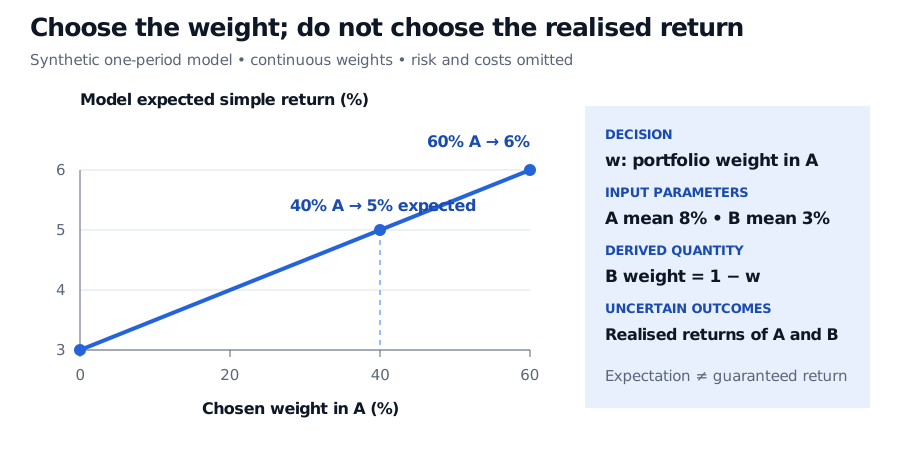
Choosing w=0.4 produces weights of 40% in A and 60% in B, with expected return 0.08(0.4)+0.03(0.6)=0.05, or 5%. This is a feasible solution; declaring the decision variable did not yet make the choice optimal.
If the objective is to maximise expected return alone, the model becomes
0≤w≤0.6max(0.03+0.05w).
The objective rises with w, so the optimal solution is w=0.6, giving expected return 6%. The cap prevents the model from putting still more in A. Risk and trading costs are omitted, so this result answers only the stated mean-only question. Neither expected return is a guaranteed realised return.
Synthetic one-period model: increasing A weight from 0% to 60% raises model expected return from 3% to 6%; 40% in A gives 5%. The chosen weight, fixed mean inputs and uncertain realised returns have separate roles.
The decision moves along the horizontal axis. The vertical axis is the model's expected return, computed from fixed mean inputs; realised returns remain uncertain. Risk and costs are omitted.
The role belongs to the problem
A quantity can change role when the question changes. Expected returns are supplied inputs in the allocation above. In an estimation problem, their estimates may be quantities fitted to data. Likewise, an option model's volatility may be fixed during pricing but chosen to minimise a calibration error. Calling it a “parameter” does not prevent it from being an optimisation variable in that second problem.
Choosing a fitted value also does not mean controlling the underlying market. The optimisation chooses a number inside a model. When a decision is made matters too: a trade selected today cannot depend on tomorrow's unobserved return; an adaptive strategy may respond later to information then available. A well-specified model states both the allowed values and the information available when each choice is made.
Unconstrained Optimisation develops this change of perspective through portfolio utility and pricing-error objectives, then explains how derivatives guide the choice of variables. The public page is a preview; full lesson access requires membership.
Sources
Gérard Cornuéjols, Javier Peña and Reha Tütüncü, Optimization Methods in Finance, second edition, §1.3, pp. 8–9 — portfolio holdings as decision variables, full-investment restrictions and mean–variance objectives; §1.1, pp. 6–7 — staged decisions under uncertainty.