Define an optimisation problem, distinguish a chosen quantity from its objective value, and solve a synthetic profit model before and after a capacity limit binds.
Optimisation
Optimisation is the process of choosing the best permitted decision according to a stated mathematical criterion. In finance, that might mean selecting portfolio weights to minimise modelled risk, choosing a trade size to maximise modelled net profit, or fitting parameters to minimise pricing error. “Best” acquires a precise meaning only after the criterion and permitted choices have been specified.
The constraints define a feasible set, often denoted F. A compact statement is
q∈FmaxΠ(q).
An optimiser is a choice attaining the best value; the word also commonly refers to the software seeking that choice. An optimal solution and an optimal value are different objects: the first is the quantity selected, the second is the profit produced by the model at that quantity. A feasible choice need not be optimal.
Maximising profit, minimising risk and minimising a pricing error are different questions. A solver cannot decide which objective expresses the user's purpose, and a constraint such as a position limit does not specify an objective by itself.
A small trade-size model, solved completely
Suppose a hypothetical trading opportunity has a known linear benefit, a quadratic size cost and a setup charge. Quantity is divisible: q can be any real number from 0 to 6 quantity units. Let modelled net profit, measured in USD, be
Π(q)=4q−21q2−3,0≤q≤6.
The coefficient 4 has units USD per quantity unit; the coefficient 1/2 has units USD per squared quantity unit. The USD 3 setup charge applies to every permitted quantity, including q=0. Thus zero quantity still records a USD 3 loss under this cost convention. An alternative in which choosing not to participate avoids that charge would require an explicitly different model.
Increasing quantity earns more gross benefit but also increases the size cost. The derivative measures marginal net profit:
Π′(q)=4−q,Π′′(q)=−1.
Their units are USD per quantity unit and USD per squared quantity unit, respectively. Marginal profit is positive below 4 and negative above 4. The interior stationary candidate is therefore q=4. Checking the endpoints gives:
Quantity (units)
Modelled net profit (USD)
0
-3.00
4
5.00
6
3.00
We can certify the answer across all permitted real quantities, rather than merely compare these three samples. Completing the square gives
Π(q)=5−21(q−4)2≤5.
The squared term is nonnegative and vanishes only at 4. Since 4 is feasible, the unique global optimum is quantity 4 units, with optimal profit USD 5. The negative second derivative throughout the interval expresses the same strict concavity. A negative second derivative at just one stationary point would establish a local maximum, without by itself comparing that point with distant feasible choices.
A binding limit changes the answer
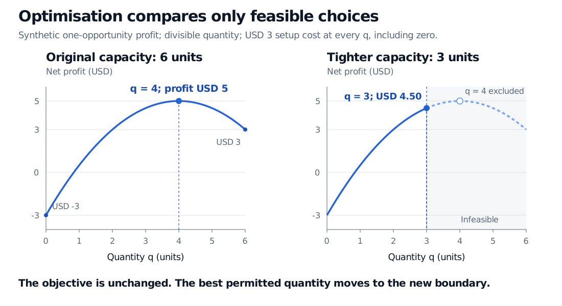
Now reduce capacity to 3 units, keeping the profit function unchanged. The new feasible set is [0,3], so quantity 4 is excluded. Marginal profit is still positive everywhere on this interval: 4−q≥1. Consequently the best permitted quantity is its upper boundary,
q∗=3,Π(3)=12−4.5−3=4.5 USD.
Original synthetic continuous trade-size model. Capacity 6 gives optimal quantity 4 and profit USD 5; endpoint profits are USD -3 at zero and USD 3 at six. Reducing capacity to 3 gives optimal quantity 3 and profit USD 4.50, while quantity 4 becomes infeasible.
The same synthetic profit curve under two capacity limits. Solid blue shows permitted quantities; the dashed portion in the right panel is excluded. The USD 3 setup cost is charged even at zero.
This is constrained optimisation. Its solution need not satisfy the unconstrained stationarity equation Π′(q)=0: at the capacity boundary, an improving move would violate the constraint. Checking only stationary points would miss the answer.
Match the method to the model
For this example, algebra supplies an exact answer. Larger problems often need numerical algorithms. Their mathematical structure determines which methods and guarantees are available:
Linear programming uses a linear objective and linear constraints. The quadratic profit above is outside that class.
Quadratic programming allows a quadratic objective with linear constraints. Maximising this concave profit is equivalent to minimising −Π, a convex quadratic, on the same interval.
Requiring whole quantities changes the feasible set to integer points. Here quantity 4 happens to remain optimal, but rounding a continuous solution is not a general solution method for integer problems.
A local optimum compares nearby feasible choices; a global optimum compares every feasible choice. For convex minimisation on a convex feasible set, every local minimum is global. General nonconvex problems lack that guarantee. A numerical stopping message should be interpreted alongside feasibility checks, the algorithm's guarantee and its stated tolerances.
Existence also needs checking. In this example the profit function is continuous on a nonempty closed, bounded interval, so a maximum is attained. Other models can have incompatible constraints, an objective that improves without bound, or a best limiting value that no feasible choice attains.
Finally, solving a model and validating its inputs are separate tasks. The USD 5 result assumes the benefit, size cost and setup charge specified above. Estimation error, uncertain fills, omitted risks or changed costs can change which real decision is attractive. A mathematical optimum is conditional on the model; it does not establish a profitable trading recommendation.
For the next mathematical step, Constrained and Convex Optimisation develops equality constraints, inequalities and global optimality conditions. To see the same framework choose model parameters instead of trades, Calibration as an Inverse Problem explains pricing-error objectives, nonuniqueness and regularisation. Both have public previews; complete lessons require membership.
Sources
Gérard Cornuéjols, Javier Peña and Reha Tütüncü, Optimization Methods in Finance, 2nd edition, Cambridge University Press, 2018, Chapter 1, especially the opening formulation and §§1.1–1.3: model components, problem classes, solution methods and financial applications.
Stephen Boyd and Lieven Vandenberghe, Convex Optimization, revised lecture slides, revised with Parth Nobel, slides 1.2–1.4 and 4.2–4.10: objectives and constraints, feasible and optimal points, and local versus global optimality in convex problems.
The trade-size scenarios and figure are original synthetic examples.