Linear programming allocates divisible quantities under linear limits. Solve a treasury example, prove its optimum with a dual bound, and see why an entire edge can tie.
Linear programming
Linear programming (LP) is optimisation of a linear objective function subject to finitely many linear equalities and inequalities. It asks how to allocate divisible quantities when benefits, costs and resource usage add at constant rates. “Programming” means choosing a plan; it does not require writing a computer program.
The decision variables are real-valued quantities. A typical maximisation form is
xmaxc⊤xsubject toAx≤b,x≥0.
Here c contains objective coefficients, each row of A describes resource usage, and b gives the corresponding limits. Other LPs use equalities, lower limits or variables allowed to be negative. Nonnegativity is a modelling choice, not part of the definition of linearity. An objective with an added constant has the same optimal allocations.
A treasury allocation, with the units kept visible
Consider a synthetic one-year treasury plan with two divisible deposits. Let x and y be the amounts placed with facilities A and B, measured in USD millions. Stipulate simple annual interest of 3% at A and 2% at B, a total funding limit of USD 4 million, and placement caps of USD 2 million and USD 3 million respectively. Cash left unplaced earns zero in this model.
Interest income, measured in units of USD 10,000 per year, is z=3x+2y. Thus the plan is
x,ymaxsubject to3x+2y,x+y≤4,x≤2,y≤3,x≥0,y≥0.
Each constraint has an economic meaning. The budget competes across facilities; the individual caps apply separately. Placing USD 2 million at A and USD 3 million at B respects both placement caps but violates the total funding limit. It is therefore not a feasible solution.
The feasible region is the intersection of all five halfplanes. Its corners and their income values are:
A: x (USD millions)
B: y (USD millions)
z (USD 10,000 per year)
0
0
0
2
0
6
2
2
10
1
3
9
0
3
6
The best corner is (2,2): USD 2 million at each facility, producing USD 100,000 of annual interest under the stipulated terms. The total budget and A cap bind. B has USD 1 million of unused placement capacity.
These are invented terms for a continuous allocation example. Repayment and interest are assumed to be performed as stipulated. The objective contains no default loss, liquidity cost, tax or other risk adjustment; solving it does not establish that the deposits are suitable investments.
Why the corner calculation works—and when corners tie
A nonempty bounded polyhedron has at least one optimal vertex for any linear objective. A linear function averages exactly along a line segment: its value at a mixture of two allocations is the same mixture of their values. Consequently, mixing worse corners cannot improve on the best corner. This is the geometric reason the table finds a global optimum, rather than just a locally attractive allocation. The general result is developed in MIT's geometry of linear optimisation notes.
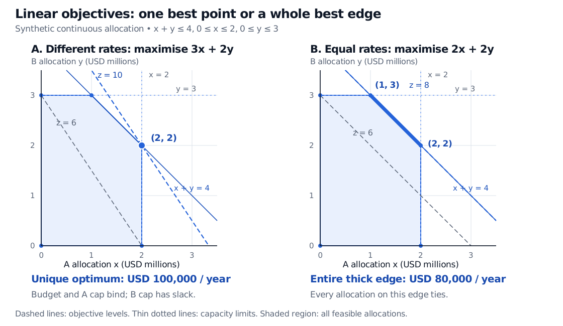
Two plots of the same synthetic treasury feasible polygon with vertices (0,0), (2,0), (2,2), (1,3) and (0,3), with both allocation axes in USD millions. Maximising 3x+2y gives the unique point (2,2), income USD 100,000 per year. Changing only the objective to 2x+2y makes the whole edge from (1,3) to (2,2) optimal, income USD 80,000 per year.
Same constraints, different objectives. Dashed lines show constant-income levels; the second panel changes A's stipulated rate to 2%, so the entire thick edge ties.
“At least one optimal vertex” does not mean every optimal solution must be a corner. If both facilities pay 2%, the objective becomes 2x+2y. Every feasible allocation with x+y=4 earns the same USD 80,000. In particular, every point on the edge joining (1,3) and (2,2) is optimal. If the objective is identically zero, every feasible point is optimal, including interior points.
The feasible region need not have positive area. Equalities can reduce it to a line segment or one point; both can still contain valid optima. An empty feasible set, by contrast, contains no admissible plan. An LP can also be feasible while its objective improves without bound. A drawing's finite viewport does not impose a genuine allocation limit.
An upper bound that proves optimality
For this example, a short inequality certifies the answer without searching the corners:
3x+2y=2(x+y)+x≤2⋅4+2=10.
Every feasible plan obeys this upper bound. The allocation (2,2) reaches it, proving optimality. Equality requires both x+y=4 and x=2, so the original optimum is unique.
This is a simple dual certificate: combine valid constraints with nonnegative weights to bound the objective. The budget receives weight 2 and A's cap weight 1; B's unused cap receives weight 0. Matching a feasible objective value with a valid bound is the central optimality test behind LP duality.
The weight on the budget also has a local resource interpretation. Raising available funds from USD 4 million to USD 5 million lets B's placement grow from USD 2 million to its USD 3 million cap, increasing annual income by USD 20,000. Beyond that point, the unchanged placement caps prevent further gains. A multiplier's marginal interpretation applies only while the relevant optimal structure remains valid.
Recognising the boundary of an LP model
Constant rates and additive usage make this example linear. A term such as xy, x2 or a portfolio variance changes the mathematical problem. Mean–variance portfolio optimisation usually has a quadratic objective, even when its budget and exposure constraints are linear.
Requiring whole lots or all-or-nothing choices introduces integer restrictions. An LP allows fractional values; an accidentally integer solution does not make it an integer-programming model. Fixed setup fees, changing rates, uncertain coefficients and risk limits also need an explicit formulation. Some can be represented using additional linear variables and constraints; others require a different problem class. A solver optimises the stated model, including its omissions.
Bertsimas, D. (2009). MIT 15.093J Optimization Methods: Lecture 5, Duality Theory I, slides 7–8 on bounds and optimality, and slide 12 on resource prices.