An objective function scores a decision. Compare return maximisation, variance minimisation and a risk-adjusted score on the same two-asset portfolio choices.
Objective function
An objective function assigns a numerical score to a choice so an optimisation problem can seek the highest or lowest score. In portfolio construction, the score might be expected return, return variance, or expected return after a risk penalty. Calling a portfolio “optimal” makes sense only after specifying that criterion and the allowed choices.
The distinction is compactly written as
x∈Fminf(x).
The decision variablex describes the choice; the objective function f maps that choice to one real number; the feasible setF contains choices permitted by the constraints. For a minimisation, lower is better. For a maximisation, higher is better. The optimal solutionx∗ is a choice, while f(x∗) is its objective value. They can have entirely different units.
An objective describes what the model rewards. It does not establish that the reward is the investor's true goal or that an optimum exists. A problem can have several optimal choices, no feasible choices, or a score that improves without attaining a best value.
One portfolio menu, two answers
Suppose a manager allocates between two hypothetical assets over one common holding period. Their simple-return moments are stipulated, rather than estimated from market data:
Input
Asset A
Asset B
Expected return
8%
4%
Return variance, decimal-return squared
0.04
0.01
Return standard deviation
20%
10%
The assets have zero covariance. Invest fraction w in A and 1−w in B, with 0≤w≤1: fully invested, no shorts, no cash asset. Ignore trading costs. The portfolio's expected return and variance are
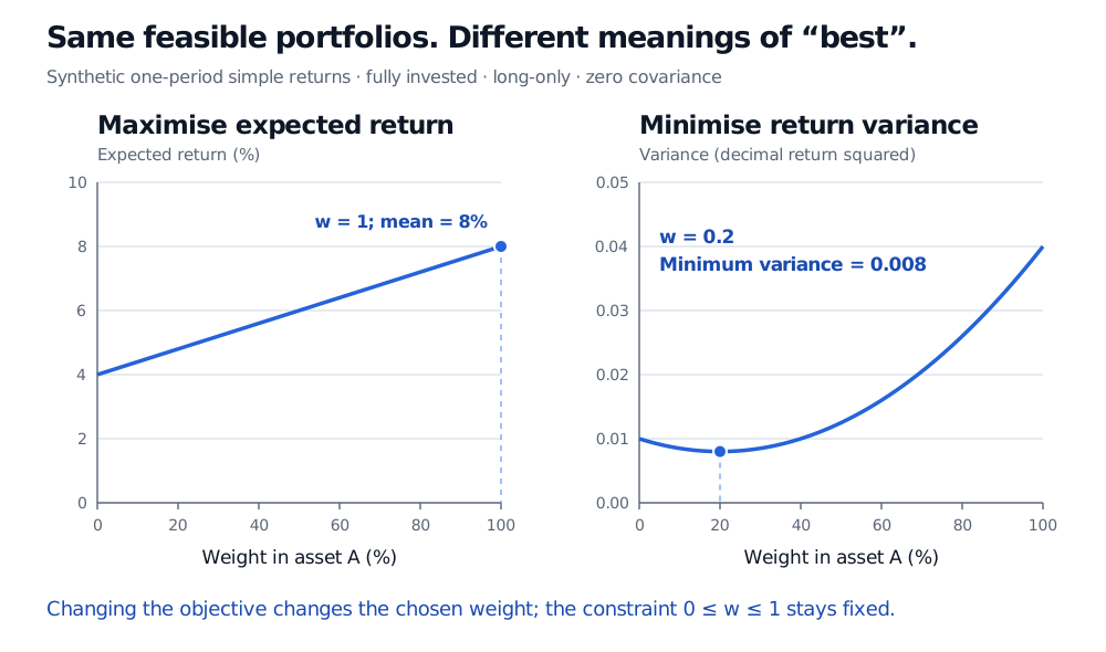
Maximise expected return. Since μ(w) increases throughout the allowed interval, choose w=1. The expected return is 8%, and the variance is 0.04. Risk has no penalty in this particular objective; the model has no reason to diversify.
Minimise variance. Rewrite the other criterion as
v(w)=0.008+0.05(w−0.2)2.
The squared term cannot be negative and vanishes at w=0.2. That feasible weight therefore gives the global minimum variance, 0.008. It invests 20% in A and 80% in B, earning an expected 4.8% with return standard deviation about 8.94%. Despite A's higher standalone variance, a modest allocation to A reduces portfolio variance because of the specified covariance.
Same synthetic long-only allocations: expected return rises from 4% to 8% and is maximised at 100% in A; variance is minimised at 20% in A, where it is 0.008.
Original one-period model comparison. The horizontal axes show the same allocation choices; the vertical axes have different units and scales. Zero covariance is an assumption, not an empirical finding.
Both answers are correct for their stated objectives. Neither changes the feasible set. In contrast, adding a cap w≤0.6 changes which allocations are allowed; under that cap, maximum expected return becomes 6.4% at w=0.6.
A trade-off needs an explicit exchange rate
Mean–variance optimisation combines return and risk into one score. A common convention is
0≤w≤1maxJλ(w),Jλ(w)=μ(w)−2λv(w),λ>0.
The parameter λ sets the risk penalty. Its numerical meaning depends on the return units and the factor-of-two convention. A higher penalty expresses a stronger preference against variance within this model; it is not an additional portfolio constraint.
For λ=5 with decimal returns,
J5′(w)=0.09−0.25w,J5′′(w)=−0.25.
The score is strictly concave, so its feasible stationary point w=0.36 is its unique maximum. The resulting expected return is 5.44%, variance is 0.00928, and score is 0.0312. The score is not a forecast return: 0.0312 includes a preference penalty; the forecast mean remains 0.0544. The risk penalty does not remove uncertainty or charge an actual fee.
Unit changes require care. Expressing returns in percentage points multiplies means by 100 and variances by 10,000. To retain the same ranking under the displayed formula, replace λ=5 by λ=0.05. Keeping the numerical penalty unchanged would describe a different trade-off. More generally, multiplying a whole objective by a positive constant or adding a constant leaves its optimisers unchanged; changing just one term's coefficient can change the answer. Maximising f is also equivalent to minimising −f.
More than one criterion does not automatically give one winner
“Maximise return and minimise risk” states two criteria. It does not specify how much return to exchange for less risk. One approach is the weighted score above. Another is to minimise variance subject to a required expected return. A third is to examine the efficient frontier: portfolios for which no feasible alternative has at least as much expected return and at most as much variance, with one strict improvement.
Choosing a frontier point still requires a preference or mandate. Two moments also omit features such as asymmetric losses, liquidity and estimation uncertainty. In a trading model, transaction costs and holding costs may belong in the objective too, with compatible units. A precisely solved objective can faithfully optimise an incomplete description of the investment problem.
For the portfolio derivations, see Mean–Variance Optimisation (public preview; full lesson requires membership).
Sources
Gérard Cornuéjols, Javier Peña and Reha Tütüncü, Optimization Methods in Finance, second edition, Cambridge University Press, 2018, Chapter 1, especially the opening model and §1.3, and Chapter 6, §§6.1–6.2. Definitions of objectives, feasible choices and optimal values; portfolio mean–variance formulations.
Stephen Boyd, Enzo Busseti, Steven Diamond, Ronald Kahn, Kwangmoo Koh, Peter Nystrup and Jan Speth, Multi-Period Trading via Convex Optimization, Foundations and Trends in Optimization 3(1), 2017. Portfolio objectives combining expected return, risk, transaction costs and holding costs.