The feasible set contains every choice satisfying all constraints. A two-asset portfolio shows intersections, a capped budget segment, convex mixtures and empty sets.
Feasible set
A feasible set is the collection of all choices that satisfy every constraint of a problem, within the stated domain. A feasible solution is one member of that collection. In portfolio construction, the set answers “which allocations are allowed?” before an objective function ranks them by return, risk or another criterion.
For a decision vector x in a domain D, a common description is
F={x∈D:gi(x)≤0 for every i,hj(x)=0 for every j}.
Here D includes the variable domain and the domains on which the problem's functions are defined. The word every matters: satisfying the budget while violating a position limit does not make a trade feasible. Equivalently, the feasible set is the intersection of the allowed sets defined by the individual requirements.
A portfolio is a segment, not a square
Consider a hypothetical portfolio containing only assets A and B. The decision variableswA,wB are continuous fractions of total portfolio wealth. Fully invested means their sum is one; long-only means neither can be negative. Add a policy cap of 60% in A:
wA+wB=1,wA≥0,wB≥0,wA≤0.6.
Eliminating wB gives the entire set:
F={(w,1−w):0≤w≤0.6}.
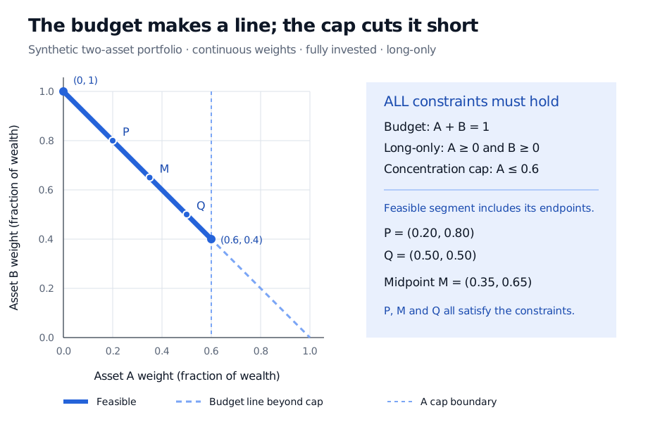
It is the closed line segment from (0,1) to (0.6,0.4). Although the vector has two coordinates, the budget leaves only one free coordinate. There is no filled area of feasible portfolios in this two-dimensional drawing. The unit square alone would allow allocations whose weights do not sum to one.
A two-asset weight diagram shows the feasible closed segment from (0, 1) to (0.6, 0.4). Feasible portfolios P=(0.2, 0.8) and Q=(0.5, 0.5) have midpoint M=(0.35, 0.65). Both axes measure fractions of total wealth.
Original synthetic allocation example. The solid blue segment satisfies the budget, long-only conditions and A cap together; the dashed continuation satisfies the budget but exceeds the cap.
Membership can be checked directly:
Allocation (wA,wB)
In the feasible set?
Reason
(0.5,0.5)
Yes
Sum is one, both weights are nonnegative, A is below 0.6.
(0.7,0.3)
No
Budget holds, but A exceeds the cap.
(0.5,0.4)
No
Weights sum to 0.9, leaving 10% unallocated in this two-asset model.
If cash were allowed as a third asset, the final row could describe part of a feasible three-asset portfolio. Feasibility is always relative to the model actually specified, including its instruments, units and domains.
Mixing allowed choices
This set is convex: every weighted average of two feasible allocations remains feasible. For example, splitting wealth equally between P=(0.2,0.8) and Q=(0.5,0.5) produces
21P+21Q=(0.35,0.65)∈F.
More generally, for t∈[0,1], the first coordinate of tP+(1−t)Q remains between 0 and 0.6, and the coordinates still sum to one. Linear equalities and non-strict linear inequalities preserve this property under intersection. Other restrictions need checking: integer share counts can rule out an average of two allowed holdings because that average may require fractional shares.
Convexity describes the available choices. It does not, by itself, select a best portfolio or guarantee that every objective has a unique optimal solution.
Empty sets and excluded endpoints
Add a minimum of 70% in A while retaining the 60% maximum. No real weight satisfies 0.7≤wA≤0.6, so F=∅. This is infeasibility: there is no allocation for an optimiser to rank. Changing the objective cannot repair contradictory constraints.
Boundary conventions also matter. The original wA≤0.6 includes (0.6,0.4); replacing it by wA<0.6 excludes that endpoint. The resulting set is still convex but is no longer closed. In numerical work, a reported constraint tolerance is an approximation rule; it should not silently change the exact mathematical set.
For the next step, Constrained and Convex Optimisation develops portfolio budget geometry, convexity and optimality conditions. Full lesson access requires membership; a public preview is available.
Sources
Cornuéjols, G., Peña, J. and Tütüncü, R. Optimization Methods in Finance, 2nd edition, §20.3 (feasible sets) and Appendix A.2 (convex sets and intersections).