A feasible solution satisfies every constraint. Check a two-asset allocation, distinguish feasibility from optimality, and interpret numerical tolerances.
Feasible solution
A feasible solution is one choice of the decision variables that lies in the problem's domain and satisfies every constraint. It is also called a feasible point. In portfolio construction, this answers a basic question: do these proposed holdings obey the model's rules?
The feasible set is the collection of all such choices; a feasible solution is one member of that collection. The word solution does not imply that the choice is best. An optimal solution must also achieve the best value of the specified objective over the feasible set.
Check a proposed allocation
Consider a synthetic, one-period portfolio with continuous weights in two fictional assets. The constraints require full investment, no short positions and at most 60% in asset A:
wA+wB=1,wA≥0,wB≥0,wA≤0.6.
These are hypothetical mandate rules. There are no transaction costs, turnover restrictions, minimum trade sizes or additional risk limits in this example.
Propose (wA,wB)=(0.4,0.6). Check each rule separately:
Rule
Substitution
Verdict
Fully invested
0.4+0.6=1
Pass
Long-only
0.4≥0 and 0.6≥0
Pass
A concentration cap
0.4≤0.6
Pass
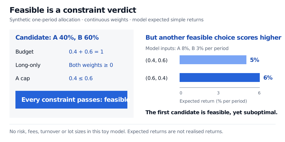
The allocation is feasible. The A cap has slack 0.6−0.4=0.2, meaning 20 percentage points of portfolio weight remain before reaching the cap. An inequality need not bind for the point to be feasible. Conversely, the equality must hold: a portfolio with weights (0.4,0.5) fails the stated budget even though neither weight is negative and the A cap is respected. Cash would need its own explicit place in the model to count as the missing allocation.
A passing allocation can still be beaten
Suppose the objective function is to maximise expected one-period simple return. Use fixed model inputs of 8% for A and 3% for B:
μp=0.08wA+0.03wB.
The feasible candidate has expected return
0.08(0.4)+0.03(0.6)=0.05=5%.
But (0.6,0.4) also satisfies every constraint and scores 0.08(0.6)+0.03(0.4)=0.06=6%. One feasible improvement is enough to prove the original candidate is not optimal.
Candidate weights A 40%, B 60% pass the budget, long-only and A-cap checks. Model expected return is 5%; another feasible allocation, A 60%, B 40%, scores 6%.
Original synthetic one-period model. Passing all three rules establishes feasibility; the return comparison disproves optimality of the 40/60 allocation. Risk and costs are omitted.
In fact, substituting wB=1−wA gives μp=0.03+0.05wA on 0≤wA≤0.6. It increases throughout that interval, so (0.6,0.4) is optimal for this particular objective and model. Different risk preferences or constraints could change that judgment. Neither 5% nor 6% is a promised realised return, and feasibility says nothing about the accuracy of the return inputs or exposure to omitted risks.
What to check in a computed result
A numerical solver's reported candidate should be checked against the original constraints, including variable bounds and domains. Record the residuals and the feasibility tolerance: for example, weights 0.4000002 and 0.6 sum to 1.0000002. The budget residual is 0.0000002, which passes a declared absolute tolerance of 0.000001 but is not exact mathematical equality. Scaling matters when different constraints use different units.
A feasible candidate demonstrates that the constraints can be satisfied. Failure to find one does not, by itself, prove the problem infeasible. Likewise, satisfying a system of linear equations does not establish uniqueness, and an equation-solving routine may return holdings that violate separate long-only or concentration restrictions.
For the next step from admissible weights to optimality conditions, Constrained and Convex Optimisation develops budget constraints, inequality constraints and the KKT conditions. Its public page is a preview; the full lesson requires membership.
Sources
Gérard Cornuéjols, Javier Peña and Reha Tütüncü, Optimization Methods in Finance, second edition, Chapter 1, “Overview of Optimization Models,” pp. 3–4 — feasible points, optimal solutions and binding constraints.