System of linear equations: Definition & Examples

A system of linear equations is a collection of equations that must hold for the same unknown quantities, with each unknown appearing only to the first power and multiplied by a fixed coefficient. A solution satisfies every equation at once. In finance, the unknowns can be instrument holdings and the equations can require those holdings to match several cash flows or risk exposures simultaneously.

A linear system can have one solution, infinitely many solutions, or no solution. Counting equations is not enough to decide which: two requirements may repeat the same information, or contradict each other.

Two instruments, two exposure targets

Suppose a desk uses two instruments, X and Y, to construct specified local exposures to two risk factors. This is an original hypothetical model at one valuation point. Each factor shock is measured in basis points (bp); positive exposure means positive first-order P&L for a positive shock to that factor, holding the other fixed.

Local sensitivity	One X contract	One Y contract	Portfolio target
Factor 1	+2	+1	+8
Factor 2	+1	−1	+1

Instrument entries are USD per bp per contract; targets are USD per bp. Let

x

and

y

be the numbers of X and Y contracts. Treat quantities as unrestricted real numbers for the algebra. Matching the targets requires

\begin{aligned} 2x+y&=8,\\ x-y&=1. \end{aligned}

These are equations between numerical values in the stated units: for example, 2 USD per bp per contract times $x$ contracts contributes $2x$ USD per bp to Factor 1. Factor 1 and Factor 2 remain separate exposure coordinates, even though their units have the same form. Neither equation is a budget constraint.

Add the equations to eliminate $y$ : $3x=9$ , hence $x=3$ . Substitution into $x-y=1$ gives $y=2$ . Check both original targets:

2(3)+2=8,\qquad 3-2=1.

Thus three X contracts and two Y contracts deliver the specified local exposures. This matches sensitivities at the chosen valuation point; it does not promise exact P&L matching for large market moves or all future states.

The matrix form packages the same information:

A\mathbf{x}=\mathbf{b},\qquad A=\begin{pmatrix}2&1\\1&-1\end{pmatrix},\quad \mathbf{x}=\begin{pmatrix}x\y\end{pmatrix},\quad \mathbf{b}=\begin{pmatrix}8\\1\end{pmatrix}.

Rows correspond to factors; columns correspond to instruments. Reading by columns, the problem asks which linear combination of the one-contract exposure vectors reaches the target. Here

3\begin{pmatrix}2\\1\end{pmatrix} +2\begin{pmatrix}1\\-1\end{pmatrix} =\begin{pmatrix}8\\1\end{pmatrix}.

A repeated requirement is not an extra restriction

Now compare three small systems. In the last two, use a different hypothetical sensitivity matrix: both instruments have Factor 1 sensitivity 1 and Factor 2 sensitivity 2, again in USD per bp per contract.

System	What elimination reveals	Solutions over real holdings
$2x+y=8$ , $x-y=1$	Adding rows gives $3x=9$	Exactly one: $(3,2)$
$x+y=3$ , $2x+2y=6$	Second row minus twice the first gives $0=0$	Infinitely many: $(t,3-t)$ for every real $t$
$x+y=3$ , $2x+2y=7$	Second row minus twice the first gives $0=1$	None

The last system asks for Factor 1 exposure 3 USD per bp and Factor 2 exposure 7 USD per bp. But every portfolio of these instruments has Factor 2 exposure exactly twice Factor 1 exposure. Meeting the first target forces the second exposure to be 6, making the requested 7 unreachable.

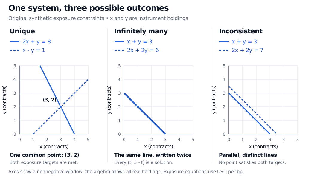
In the row picture, each equation with a nonzero coefficient row in two unknowns describes a line in the holdings plane. Solving the system means finding their common points. Distinct intersecting lines give one solution; coincident lines give infinitely many; parallel distinct lines give none.

Three holdings-plane diagrams. The lines 2x plus y equals 8 and x minus y equals 1 meet at 3 X contracts and 2 Y contracts. The equations x plus y equals 3 and 2x plus 2y equals 6 coincide. Replacing the second target with 7 creates a parallel distinct line and no solution. Both axes are contract quantities; exposure equations use USD per bp.

Original synthetic exposure examples. Axes show holdings, not factor shocks. The displayed nonnegative window illustrates unrestricted real systems; it does not impose a trading restriction.

The general test: reachability, then uniqueness

For

m

equations and

n

unknowns,

A

has shape

m\times n

, the holdings vector has

n

entries, and the target has

m

. An exact solution exists precisely when

\mathbf{b}

lies in the span of the columns of

A

. This is consistency: the instruments can produce the target.

Gaussian elimination applies reversible row operations to the augmented matrix $[A\mid\mathbf{b}]$ . Apply each operation to the target column too. A resulting row $0=c$ with $c\ne0$ proves inconsistency. A row $0=0$ is redundant; it does not by itself prove that there are free holdings.

Once consistency is established, matrix rank decides uniqueness. If the rank is

n

, there are no free variables and the solution is unique. If rank is smaller than

n

, there are

n-\operatorname{rank}(A)

free variables and infinitely many real solutions. Equivalently, all solutions are

\mathbf{x}=\mathbf{x}_p+\mathbf{z},\qquad A\mathbf{z}=\mathbf{0},

where

\mathbf{x}_p

is any one solution and

\mathbf{z}

ranges over the null space. Such adjustments leave the modelled outputs unchanged. They need not have zero cost or zero exposure to risks omitted from

A

. MIT's lecture summary develops this particular-solution-plus-null-space description.

For square

A

, a nonzero determinant guarantees one solution for every target. The first example has determinant

2(-1)-1(1)=-3

. Its inverse therefore exists, although numerical implementations normally solve the system directly using a suitable factorisation rather than explicitly forming the inverse. A theoretically unique solution can still be sensitive to small input changes when the system is poorly conditioned.

A solution is not yet an executable portfolio

The algebra answers an equality problem under its declared domain. Economic feasibility adds requirements. A cap of at most two X contracts rules out the unique solution

(3,2)

above; no other holdings can meet those same two exposure targets. In the redundant example, long-only holdings restrict the family to

0\le t\le3

, leaving a continuum. Integer contracts would instead retain just

(0,3)

(1,2)

(2,1)

and

(3,0)

. The three-outcome classification applies to unrestricted real linear systems, not to every constrained trading problem.

Budgets, margin, short-sale permissions, lot sizes, liquidity and trading costs must be added explicitly. Choosing the cheapest or lowest-risk portfolio among many solutions is an optimisation problem. If no exact solution exists, least squares can choose an approximation under a specified error metric; it does not make the original equations consistent. Mixing differently scaled exposure rows without a deliberate weighting can make that approximation economically misleading.

For a longer geometric treatment, Systems of Linear Equations and the Row Picture develops line and plane intersections. The Complete Solution to Ax = b extends the analysis to rank and free variables. Both have public previews; full lessons require membership.

Sources

Gilbert Strang, Introduction to Linear Algebra, 5th edition (2016), §2.1, “Vectors and Linear Equations,” and §3.3, “The Complete Solution to Ax = b,” pp. 150–155.
MIT OpenCourseWare, 18.06SC Linear Algebra, Fall 2011: “Solving Ax = b: Row Reduced Form R,” lecture summary — consistency, particular solutions, null space and rank. Financial examples and figure are original.

Two instruments, two exposure targets

A repeated requirement is not an extra restriction

The general test: reachability, then uniqueness

A solution is not yet an executable portfolio

Sources

Related terms

Determinant

Least squares

Linear combination

Matrix

Matrix inverse

Matrix rank

Null space

Span