Matrix rank: Definition & Examples

Matrix rank is the number of independent directions in a matrix's columns. Equivalently, it is the dimension of their span, the number of independent rows, and the number of pivots after exact row reduction. A matrix with many entries can have very little independent information.

For a quant, rank answers a concrete question: how many distinct exposure directions can these instruments control? Three hedge instruments may offer three ways to trade the same risk, rather than three risks that can be adjusted separately.

Three instruments, one hedge direction

Consider a synthetic local model with two interest-rate factors. A shock to either factor is measured in basis points. Each column below records one contract's sensitivity to the two factors, in USD per basis point per contract:

A=\begin{bmatrix}1&2&3\\2&4&6\end{bmatrix}.

Call the instruments A, B and C, in column order. If their quantities are $\mathbf q=(q_1,q_2,q_3)^{\mathsf T}$ contracts, their combined exposure is

\mathbf e=A\mathbf q =\begin{bmatrix}q_1+2q_2+3q_3\\2q_1+4q_2+6q_3\end{bmatrix} =\begin{bmatrix}s\\2s\end{bmatrix}, \qquad s=q_1+2q_2+3q_3.

Both components of $\mathbf e$ are in USD per basis point. For small factor shocks $\Delta r_1,\Delta r_2$ , measured in basis points, the model gives $\Delta V\approx e_1\Delta r_1+e_2\Delta r_2$ USD. It describes local first-order exposure; it does not give a globally exact payoff hedge.

The second and third columns are two and three times the first. All three vectors lie on the same line, so the rank is 1. Adding more of B or C cannot create exposure outside that line. The rows tell the same story: the second row is twice the first, so the factor-2 exposure is always twice the factor-1 exposure.

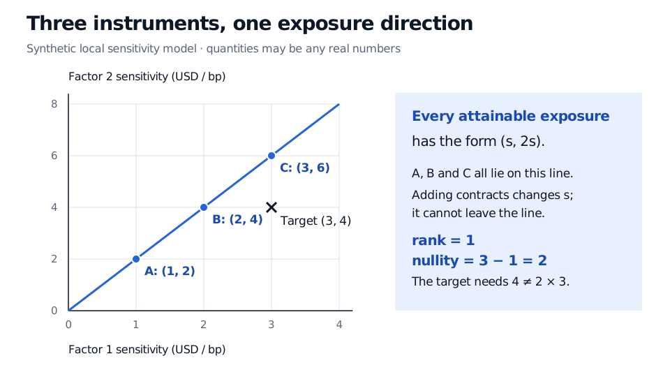
Instrument sensitivities A (1, 2), B (2, 4) and C (3, 6), in USD per bp for one contract, lie on the line e2 equals 2e1. All real-valued positions stay on this line. Target exposure (3, 4) USD per bp is outside it. Rank is 1 and nullity is 2.

Original synthetic sensitivity model. Columns show one-contract exposures; the line shows all exposures attainable with unrestricted real contract quantities. This is a local exposure map, not a terminal-payoff diagram.

A desired exposure of $(3,4)^{\mathsf T}$ USD per basis point is impossible: its second component is not twice its first. Thus a portfolio with exposure $(-3,-4)^{\mathsf T}$ cannot be neutralised in both modelled factors with these instruments alone.

An exposure of $(5,10)^{\mathsf T}$ is attainable, but the quantities are not unique. For any real $u,v$ ,

\mathbf q=\begin{bmatrix}5-2u-3v\u\v\end{bmatrix} \quad\Longrightarrow\quad A\mathbf q=\begin{bmatrix}5\\10\end{bmatrix}.

For example, five A contracts work, as do one A and two B contracts. These positions have the same two sensitivities; their prices, liquidity, funding requirements and exposures to omitted factors can differ.

Count the pivots, then count what is left

Subtract twice the first row from the second:

\begin{bmatrix}1&2&3\\2&4&6\end{bmatrix} \longrightarrow \begin{bmatrix}1&2&3\\0&0&0\end{bmatrix}.

There is one pivot, confirming rank 1. Row operations preserve rank and the solutions of the homogeneous equation $A\mathbf q=\mathbf0$ . They need not preserve the column space as the same geometric subset of the output coordinates: use the original columns when describing the original attainable exposures.

The null space contains the positions with zero modelled exposure. Here it is

\ker A=\left\{ u\begin{bmatrix}-2\\1\\0\end{bmatrix} +v\begin{bmatrix}-3\\0\\1\end{bmatrix}:u,v\in\mathbb R \right\}.

Both displayed vectors map to zero, and they are linearly independent. The null space therefore has dimension 2. This is the rank-nullity theorem: for an

m\times n

matrix of rank

r

\dim(\ker A)=n-r.

In this example,

3-1=2

independent position adjustments leave the modelled exposure unchanged. They are zero-sensitivity positions, not necessarily zero-payoff trades or arbitrage opportunities. The two-factor first-order model alone cannot establish either claim.

What “full rank” promises

Rank always satisfies

0\le r\le\min(m,n)

. The zero matrix has rank 0. A matrix is full rank when

r=\min(m,n)

, but rectangular shape matters:

Condition for an $m\times n$ matrix	Meaning for $A\mathbf q=\mathbf b$ , with unrestricted real quantities
Full column rank: $r=n$	A reachable target has a unique position vector. Some targets can remain unreachable when $m>n$ .
Full row rank: $r=m$	Every target in $\mathbb R^m$ is reachable. When $n>m$ , each has infinitely many position vectors.
Square and full rank: $m=n=r$	Every target has exactly one solution; the matrix inverse exists.

For a particular target, reachability can be tested by appending it as a column:

\operatorname{rank}([A\mid\mathbf b])=\operatorname{rank}(A)

. An extra pivot in the augmented matrix signals an inconsistent system. A determinant test applies directly only to square matrices; our

2\times3

matrix has no determinant of its own.

These are algebraic results. Short-sale restrictions, integer lots, collateral or position limits can shrink the feasible exposure set even when the matrix has full row rank. Rank also depends on which factors or scenarios were included; it cannot certify coverage of risks absent from the model.

A tiny change can alter exact rank

Change just the bottom-right entry from $6$ to $6.000001$ :

A_\varepsilon= \begin{bmatrix}1&2&3\\2&4&6+\varepsilon\end{bmatrix}, \qquad \varepsilon=10^{-6}.

The square submatrix formed from columns 1 and 3 has determinant

1(6+\varepsilon)-3(2)=\varepsilon\ne0

. Those columns are independent, so exact rank is now 2. This statement treats the entered finite decimals as exact rational numbers; it does not claim that measured economic sensitivities are known to six decimal places.

The formerly unreachable target $(3,4)^{\mathsf T}$ now has a solution. Setting $q_2=0$ gives

q_3=\frac{4-2(3)}{\varepsilon}=-2{,}000{,}000, \qquad q_1=3-3q_3=6{,}000{,}003.

Huge offsetting positions exploit the tiny difference between almost redundant columns. If the true bottom-right sensitivity were $6$ instead, these same quantities would produce $(3,6)^{\mathsf T}$ , missing the second target by 2 USD per basis point. Exact reachability does not promise a stable or feasible hedge.

Numerical rank adds an explicit threshold. Using a singular value decomposition, one common rule counts singular values satisfying $\sigma_i>\tau\sigma_{\max}$ for a chosen relative tolerance $\tau$ . For this entered matrix, the smaller-to-larger singular-value ratio is about $3.19\times10^{-8}$ :

Relative tolerance $\tau$	Numerical rank under that rule
$10^{-10}$	2
$10^{-6}$	1

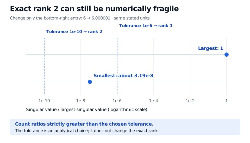
For the synthetic perturbed matrix with bottom-right entry 6.000001, the singular-value ratios are 1 and approximately 3.19e-8. Relative tolerance 1e-10 counts both, giving numerical rank 2. Relative tolerance 1e-6 counts only the largest, giving numerical rank 1. Exact rank remains 2.

Original calculation for the stated matrix and units. The logarithmic axis compares singular values with the largest one. The thresholds illustrate two analytical choices, not two conflicting exact-rank results.

Numerical rank therefore needs its tolerance and scaling reported alongside it. Changing factor units or contract sizing can change singular-value ratios even though nonzero row or column rescaling leaves exact rank unchanged. Tolerances should reflect the intended calculation and uncertainty in the inputs; machine rounding is only one source of error. NumPy's rank documentation explains this distinction. A single computed rank number cannot settle whether the second hedge direction is economically usable.

For a fuller treatment, Kernel, Image, and the Rank-Nullity Theorem connects attainable outputs and redundant inputs to injectivity and surjectivity. The public page is a preview; the full lesson requires membership.

Sources

Gilbert Strang, Introduction to Linear Algebra, fifth edition (Wellesley–Cambridge Press, 2016), §3.2, especially pp. 139–141: pivots, rank-one matrices and free variables.
MIT OpenCourseWare, “Solving Ax = 0: Pivot Variables, Special Solutions”, 18.06SC Linear Algebra, Fall 2011, Gilbert Strang.
NumPy Developers, numpy.linalg.matrix_rank: singular-value thresholds and tolerance choices for uncertain data.

Three instruments, one hedge direction

Count the pivots, then count what is left

What “full rank” promises

A tiny change can alter exact rank

Sources

Related terms

Determinant

Dimension

Linear independence

Matrix inverse

Null space

Span

Vector